6.4.3. Hyperparameter Tuning: Finding Optimal Settings#
You’ve trained a Random Forest with default parameters. Performance: 85%. But what if n_estimators=200 gives 92%?
Hyperparameters are settings you choose before training (unlike parameters learned during training). Examples:
Tree depth in Decision Trees
Number of neighbors in KNN
Learning rate in Neural Networks
Regularization strength
Problem: How to find the best settings?
Let’s explore systematic tuning strategies from simple to advanced!
6.4.3.1. Hyperparameters vs Parameters#
Key distinction:
Parameters: Learned from data (e.g., weights, coefficients)
Hyperparameters: Set before training (e.g., learning rate, tree depth)
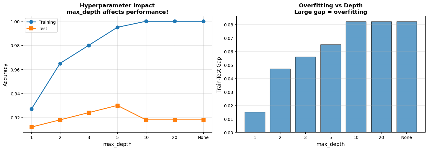
6.4.3.2. Example: Impact of Hyperparameters#
Let’s see how much hyperparameters matter!
# Load data
cancer = load_breast_cancer()
X_cancer = cancer.data
y_cancer = cancer.target

X_train, X_test, y_train, y_test = train_test_split(
    X_cancer, y_cancer, test_size=0.3, random_state=42, stratify=y_cancer
)

# Try different max_depth values
depths = [1, 2, 3, 5, 10, 20, None]
results = []

for depth in depths:
    dt = DecisionTreeClassifier(max_depth=depth, random_state=42)
    dt.fit(X_train, y_train)
    results.append({
        'max_depth': str(depth),
        'Train Accuracy': round(dt.score(X_train, y_train), 3),
        'Test Accuracy':  round(dt.score(X_test,  y_test),  3),
    })

df_results = pd.DataFrame(results)
display(df_results)

# Visualize
fig, axes = plt.subplots(1, 2, figsize=(14, 5))
depth_labels = [str(d) for d in depths]
x_pos = range(len(depth_labels))

axes[0].plot(x_pos, df_results['Train Accuracy'], 'o-', linewidth=2, markersize=8, label='Training')
axes[0].plot(x_pos, df_results['Test Accuracy'],  's-', linewidth=2, markersize=8, label='Test')
axes[0].set_xticks(x_pos)
axes[0].set_xticklabels(depth_labels)
axes[0].set_xlabel('max_depth', fontsize=12)
axes[0].set_ylabel('Accuracy', fontsize=12)
axes[0].set_title('Hyperparameter Impact\nmax_depth affects performance!', fontsize=13, fontweight='bold')
axes[0].legend()
axes[0].grid(True, alpha=0.3)

gaps = df_results['Train Accuracy'] - df_results['Test Accuracy']
axes[1].bar(x_pos, gaps, alpha=0.7, edgecolor='black')
axes[1].set_xticks(x_pos)
axes[1].set_xticklabels(depth_labels)
axes[1].set_xlabel('max_depth', fontsize=12)
axes[1].set_ylabel('Train-Test Gap', fontsize=12)
axes[1].set_title('Overfitting vs Depth\nLarge gap = overfitting', fontsize=13, fontweight='bold')
axes[1].grid(True, alpha=0.3, axis='y')

plt.tight_layout()
plt.show()
| max_depth | Train Accuracy | Test Accuracy | |
|---|---|---|---|
| 0 | 1 | 0.927 | 0.912 |
| 1 | 2 | 0.965 | 0.918 |
| 2 | 3 | 0.980 | 0.924 |
| 3 | 5 | 0.995 | 0.930 |
| 4 | 10 | 1.000 | 0.918 |
| 5 | 20 | 1.000 | 0.918 |
| 6 | None | 1.000 | 0.918 |
6.4.3.3. Grid Search: Exhaustive Search#
Grid Search: Try all combinations in a grid
How it works:
Define hyperparameter grid (e.g., depth: [3, 5, 10], min_samples: [2, 5, 10])
Try all 3×3 = 9 combinations
Use cross-validation to evaluate each
Pick best combination
Pros: Guaranteed to find best in grid Cons: Slow (exponential in # of hyperparameters)
param_grid = {
    'max_depth': [3, 5, 10, 20],
    'min_samples_split': [2, 5, 10],
    'min_samples_leaf': [1, 2, 4]
}

dt_base = DecisionTreeClassifier(random_state=42)
start = time.time()
grid_search = GridSearchCV(
    dt_base, param_grid, cv=5, scoring='accuracy', n_jobs=-1, return_train_score=True
)
grid_search.fit(X_train, y_train)
elapsed = time.time() - start
Traceback (most recent call last):
  File "/home/runner/.local/share/uv/python/cpython-3.13.12-linux-x86_64-gnu/lib/python3.13/multiprocessing/resource_tracker.py", line 371, in main
    raise ValueError(
        f'Cannot register {name} for automatic cleanup: '
        f'unknown resource type {rtype}')
ValueError: Cannot register /dev/shm/joblib_memmapping_folder_2335_4ed70938c4e542b5b694e7b335bb95b4_b3c946b4193a43ada0f37b902e1553ef for automatic cleanup: unknown resource type folder
Traceback (most recent call last):
  File "/home/runner/.local/share/uv/python/cpython-3.13.12-linux-x86_64-gnu/lib/python3.13/multiprocessing/resource_tracker.py", line 371, in main
    raise ValueError(
        f'Cannot register {name} for automatic cleanup: '
        f'unknown resource type {rtype}')
ValueError: Cannot register /loky-2335-cpqfpw7l for automatic cleanup: unknown resource type semlock
Traceback (most recent call last):
  File "/home/runner/.local/share/uv/python/cpython-3.13.12-linux-x86_64-gnu/lib/python3.13/multiprocessing/resource_tracker.py", line 371, in main
    raise ValueError(
        f'Cannot register {name} for automatic cleanup: '
        f'unknown resource type {rtype}')
ValueError: Cannot register /loky-2335-_n0yy2go for automatic cleanup: unknown resource type semlock
Traceback (most recent call last):
  File "/home/runner/.local/share/uv/python/cpython-3.13.12-linux-x86_64-gnu/lib/python3.13/multiprocessing/resource_tracker.py", line 371, in main
    raise ValueError(
        f'Cannot register {name} for automatic cleanup: '
        f'unknown resource type {rtype}')
ValueError: Cannot register /loky-2335-7w68h_o3 for automatic cleanup: unknown resource type semlock
Traceback (most recent call last):
  File "/home/runner/.local/share/uv/python/cpython-3.13.12-linux-x86_64-gnu/lib/python3.13/multiprocessing/resource_tracker.py", line 371, in main
    raise ValueError(
        f'Cannot register {name} for automatic cleanup: '
        f'unknown resource type {rtype}')
ValueError: Cannot register /loky-2335-x1bjip65 for automatic cleanup: unknown resource type semlock
Traceback (most recent call last):
  File "/home/runner/.local/share/uv/python/cpython-3.13.12-linux-x86_64-gnu/lib/python3.13/multiprocessing/resource_tracker.py", line 371, in main
    raise ValueError(
        f'Cannot register {name} for automatic cleanup: '
        f'unknown resource type {rtype}')
ValueError: Cannot register /loky-2335-0jubb668 for automatic cleanup: unknown resource type semlock
Traceback (most recent call last):
  File "/home/runner/.local/share/uv/python/cpython-3.13.12-linux-x86_64-gnu/lib/python3.13/multiprocessing/resource_tracker.py", line 371, in main
    raise ValueError(
        f'Cannot register {name} for automatic cleanup: '
        f'unknown resource type {rtype}')
ValueError: Cannot register /loky-2335-i4j3gg6t for automatic cleanup: unknown resource type semlock
Traceback (most recent call last):
  File "/home/runner/.local/share/uv/python/cpython-3.13.12-linux-x86_64-gnu/lib/python3.13/multiprocessing/resource_tracker.py", line 371, in main
    raise ValueError(
        f'Cannot register {name} for automatic cleanup: '
        f'unknown resource type {rtype}')
ValueError: Cannot register /dev/shm/joblib_memmapping_folder_2335_4ed70938c4e542b5b694e7b335bb95b4_67a0a4ecf8af411d8fcec23d6a216b14 for automatic cleanup: unknown resource type folder
Traceback (most recent call last):
  File "/home/runner/.local/share/uv/python/cpython-3.13.12-linux-x86_64-gnu/lib/python3.13/multiprocessing/resource_tracker.py", line 371, in main
    raise ValueError(
        f'Cannot register {name} for automatic cleanup: '
        f'unknown resource type {rtype}')
ValueError: Cannot register /loky-2335-18jralxc for automatic cleanup: unknown resource type semlock
Traceback (most recent call last):
  File "/home/runner/.local/share/uv/python/cpython-3.13.12-linux-x86_64-gnu/lib/python3.13/multiprocessing/resource_tracker.py", line 371, in main
    raise ValueError(
        f'Cannot register {name} for automatic cleanup: '
        f'unknown resource type {rtype}')
ValueError: Cannot register /loky-2335-khe8034b for automatic cleanup: unknown resource type semlock
Traceback (most recent call last):
  File "/home/runner/.local/share/uv/python/cpython-3.13.12-linux-x86_64-gnu/lib/python3.13/multiprocessing/resource_tracker.py", line 371, in main
    raise ValueError(
        f'Cannot register {name} for automatic cleanup: '
        f'unknown resource type {rtype}')
ValueError: Cannot register /dev/shm/joblib_memmapping_folder_2335_4ed70938c4e542b5b694e7b335bb95b4_67a0a4ecf8af411d8fcec23d6a216b14 for automatic cleanup: unknown resource type folder
---------------------------------------------------------------------------
TypeError                                 Traceback (most recent call last)
Cell In[4], line 1
----> 1 glue('gs-elapsed',   float(round(elapsed, 2), 2),                       display=False)
      2 glue('gs-cv-score',  float(round(grid_search.best_score_, 3), 2),       display=False)
      3 glue('gs-test-score',float(round(grid_search.score(X_test, y_test), 3), 2), display=False)

TypeError: float expected at most 1 argument, got 2
cv_results = pd.DataFrame(grid_search.cv_results_)
top_5 = cv_results.nlargest(5, 'mean_test_score')[
    ['param_max_depth', 'param_min_samples_split', 'param_min_samples_leaf',
     'mean_test_score', 'std_test_score']
].round(4)
display(top_5)
Grid Search completed in seconds. Best CV accuracy: , test accuracy: .
6.4.3.4. Visualizing Grid Search Results#
results_subset = cv_results[cv_results['param_min_samples_leaf'] == 1]

depths_unique = sorted(results_subset['param_max_depth'].unique())
splits_unique = sorted(results_subset['param_min_samples_split'].unique())

# Create heatmap matrix
heatmap_data = np.zeros((len(splits_unique), len(depths_unique)))

for i, split in enumerate(splits_unique):
    for j, depth in enumerate(depths_unique):
        mask = ((results_subset['param_max_depth'] == depth) &
                (results_subset['param_min_samples_split'] == split))
        score = results_subset[mask]['mean_test_score'].values[0]
        heatmap_data[i, j] = score

# Plot
fig, axes = plt.subplots(1, 2, figsize=(14, 5))

# Heatmap
im = axes[0].imshow(heatmap_data, cmap='RdYlGn', aspect='auto',
                    vmin=0.9, vmax=1.0)
axes[0].set_xticks(range(len(depths_unique)))
axes[0].set_yticks(range(len(splits_unique)))
axes[0].set_xticklabels(depths_unique)
axes[0].set_yticklabels(splits_unique)
axes[0].set_xlabel('max_depth', fontsize=12)
axes[0].set_ylabel('min_samples_split', fontsize=12)
axes[0].set_title('Grid Search Heatmap\n(Darker green = better)',
                  fontsize=13, fontweight='bold')

# Add text annotations
for i in range(len(splits_unique)):
    for j in range(len(depths_unique)):
        text = axes[0].text(j, i, f'{heatmap_data[i, j]:.3f}',
                          ha="center", va="center", color="black",
                          fontsize=9)

plt.colorbar(im, ax=axes[0], label='CV Accuracy')

# Score distribution
all_scores = cv_results['mean_test_score']

axes[1].hist(all_scores, bins=20, alpha=0.7, edgecolor='black')
axes[1].axvline(grid_search.best_score_, color='red', linestyle='--',
               linewidth=2, label=f'Best: {grid_search.best_score_:.3f}')
axes[1].set_xlabel('CV Accuracy', fontsize=12)
axes[1].set_ylabel('Frequency', fontsize=12)
axes[1].set_title('Distribution of Hyperparameter Combinations',
                  fontsize=13, fontweight='bold')
axes[1].legend()
axes[1].grid(True, alpha=0.3, axis='y')

plt.tight_layout()
plt.show()
6.4.3.5. Random Search: Efficient Alternative#
Random Search: Sample random combinations from distributions
Why it works:
Not all hyperparameters equally important
Random search explores more values for important ones
Often finds good solution faster than grid search
When to use: Large search space, limited computation
param_distributions = {
    'max_depth':          randint(3, 30),
    'min_samples_split':  randint(2, 20),
    'min_samples_leaf':   randint(1, 10),
    'max_features':       uniform(0.1, 0.9),
}

start_rs = time.time()
random_search = RandomizedSearchCV(
    dt_base, param_distributions, n_iter=50,
    cv=5, scoring='accuracy', n_jobs=-1, random_state=42, return_train_score=True
)
random_search.fit(X_train, y_train)
elapsed_random = time.time() - start_rs

best_params_df = pd.DataFrame([
    {'Hyperparameter': k, 'Best Value': round(v, 3) if isinstance(v, float) else v}
    for k, v in random_search.best_params_.items()
])
display(best_params_df)

comparison_df = pd.DataFrame([
    {'Method': 'Grid Search',   'Time (s)': round(elapsed, 2),        'Best CV Score': round(grid_search.best_score_,   3)},
    {'Method': 'Random Search', 'Time (s)': round(elapsed_random, 2), 'Best CV Score': round(random_search.best_score_, 3)},
])
display(comparison_df)
6.4.3.6. Nested Cross-Validation: Unbiased Evaluation#
Problem: Reporting CV score from GridSearchCV is biased (overfitted to validation set)
Solution: Nested CV
Outer loop: Estimate true performance
Inner loop: Hyperparameter tuning
# NON-nested (biased estimate) — GridSearchCV wrapped in cross_val_score
grid_search_nested = GridSearchCV(dt_base, param_grid, cv=5)
cv_scores_biased = cross_val_score(grid_search_nested, X_train, y_train, cv=5)

# True nested CV uses the outer loop for performance, inner for tuning
# (sklearn does this correctly when you pass a GridSearchCV to cross_val_score)
nested_df = pd.DataFrame([
    {'Approach': 'Non-nested (biased)',    'Mean CV Accuracy': round(cv_scores_biased.mean(), 3), 'Std': round(cv_scores_biased.std(), 3), 'Note': 'Optimistic bias'},
    {'Approach': 'Best practice: nested', 'Mean CV Accuracy': '—',                               'Std': '—',                              'Note': 'Outer loop = performance, inner loop = tuning'},
])
display(nested_df)
Warning
Never report GridSearchCV.best_score_ as final performance — it is the score on the same folds used to select the hyperparameters. Use a held-out test set or proper nested CV instead.
6.4.3.7. Real-World Example: Random Forest Tuning#
Let’s tune a Random Forest with multiple hyperparameters!
digits = load_digits()
X_digits, y_digits = digits.data, digits.target

X_train_rf, X_test_rf, y_train_rf, y_test_rf = train_test_split(
    X_digits, y_digits, test_size=0.3, random_state=42, stratify=y_digits
)

rf_default = RandomForestClassifier(random_state=42)
rf_default.fit(X_train_rf, y_train_rf)
default_score = rf_default.score(X_test_rf, y_test_rf)

param_dist_rf = {
    'n_estimators': [50, 100, 200],
    'max_depth': [10, 20, 30, None],
    'min_samples_split': [2, 5, 10],
    'min_samples_leaf': [1, 2, 4],
    'max_features': ['sqrt', 'log2', None]
}

random_search_rf = RandomizedSearchCV(
    RandomForestClassifier(random_state=42),
    param_dist_rf, n_iter=100, cv=3, scoring='accuracy', n_jobs=-1, random_state=42
)
random_search_rf.fit(X_train_rf, y_train_rf)
tuned_score = random_search_rf.score(X_test_rf, y_test_rf)

glue('rf-default-score', round(default_score, 3), display=False)
glue('rf-tuned-score',   round(tuned_score,   3), display=False)

display(pd.DataFrame([
    {'Model': 'Default Random Forest', 'Test Accuracy': round(default_score, 3)},
    {'Model': 'Tuned Random Forest',   'Test Accuracy': round(tuned_score,   3)},
    {'Model': 'Best params',           'Test Accuracy': str(random_search_rf.best_params_)},
]))
Tuning lifts accuracy from to .
6.4.3.8. Key Takeaways#
Important
Remember These Points:
Hyperparameters Matter
Can double performance!
Default rarely optimal
Always tune systematically
Grid Search
Exhaustive search
Use for small grids (< 100 combos)
Guaranteed to find best in grid
Random Search
Sample random combinations
More efficient for large spaces
Often finds good solution faster
Search Space Design
Start broad, then narrow
Use domain knowledge
Log scale for learning rates
Validation Strategy
Use CV (stratified if imbalanced)
Nested CV for unbiased estimates
Never tune on test set!
Computational Efficiency
Parallel execution (n_jobs=-1)
Random Search for large spaces
Reduce CV folds if needed
Reporting
Report test set performance
Document best hyperparameters
Include search time