6.1.4. Model Complexity

In machine learning, one of the most important concepts is model complexity - how flexible or expressive a model can be. Understanding complexity is crucial because it directly determines whether your model will succeed or fail. In this section, we’ll build intuition for what complexity means and why it matters.

6.1.4.1. What is Model Complexity?

Imagine you’re trying to draw a curve through some points:

• Simple approach: Draw a straight line

• Complex approach: Draw a wiggly curve that touches every point

Which is better? It depends! This is the essence of model complexity.

Model complexity refers to a model’s capacity to fit various patterns:

• Simple models: Limited flexibility, strong assumptions

• Complex models: High flexibility, few assumptions

import numpy as np
import matplotlib.pyplot as plt
from sklearn.linear_model import LinearRegression
from sklearn.preprocessing import PolynomialFeatures
from sklearn.pipeline import make_pipeline
from myst_nb import glue

# Generate data with some noise
np.random.seed(42)
X = np.sort(np.random.uniform(0, 10, 30)).reshape(-1, 1)
y = 2 + 3*X.ravel() - 0.5*X.ravel()**2 + np.random.normal(0, 5, 30)

# Create models of different complexity
models = {
    'Simple (Linear)': make_pipeline(PolynomialFeatures(1), LinearRegression()),
    'Medium (Quadratic)': make_pipeline(PolynomialFeatures(2), LinearRegression()),
    'Complex (Degree 9)': make_pipeline(PolynomialFeatures(9), LinearRegression())
}

Show code cell source

Hide code cell source

# Fit and plot
fig, axes = plt.subplots(1, 3, figsize=(16, 4))
X_plot = np.linspace(0, 10, 200).reshape(-1, 1)

for ax, (name, model) in zip(axes, models.items()):
    model.fit(X, y)
    y_plot = model.predict(X_plot)

    ax.scatter(X, y, color='blue', s=60, alpha=0.6, label='Data')
    ax.plot(X_plot, y_plot, color='red', linewidth=2, label='Model')
    ax.set_xlabel('X', fontsize=12)
    ax.set_ylabel('y', fontsize=12)
    ax.set_title(name, fontsize=13, fontweight='bold')
    ax.legend()
    ax.grid(True, alpha=0.3)
    ax.set_ylim([y.min()-5, y.max()+5])

plt.tight_layout()
plt.show()

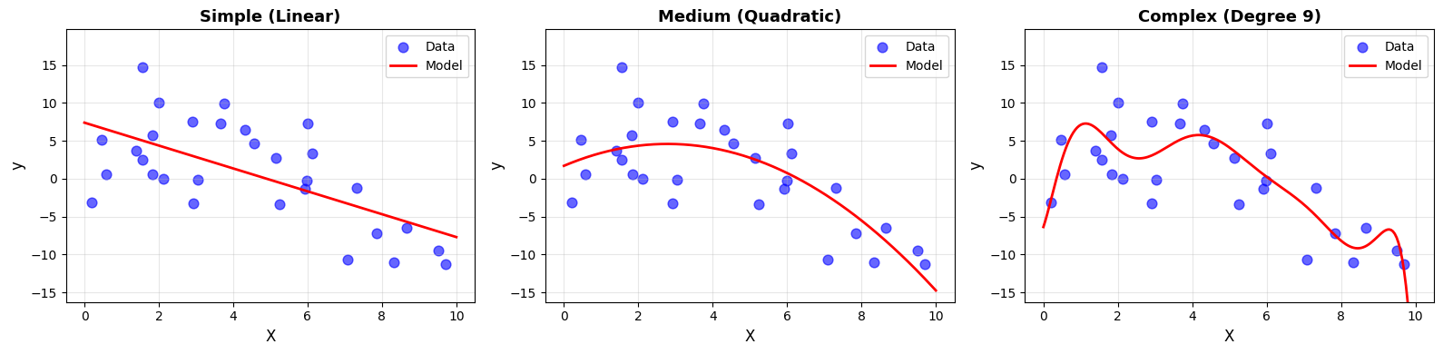
Notice how the complexity affects the fit:

• Simple: Smooth but misses curvature

• Medium: Captures underlying pattern

• Complex: Wiggly, follows noise

6.1.4.2. Defining Complexity

Model complexity describes how expressive a model is. A more complex model can represent richer patterns, but it also carries a higher risk of overfitting.

There are three closely related ways to understand complexity.

Number of Parameters

The simplest measure of complexity is the number of learnable parameters.

More parameters → more expressive power

from sklearn.tree import DecisionTreeRegressor
from sklearn.neural_network import MLPRegressor

models_params = [
    ("Linear (y = mx + b)", LinearRegression(), X, "2 parameters"),
    ("Degree-5 Polynomial", make_pipeline(PolynomialFeatures(5), LinearRegression()), X, "6 parameters"),
    ("Decision Tree (depth=10)", DecisionTreeRegressor(max_depth=10, random_state=42), X, "Up to 1024 leaf nodes"),
    ("Neural Net (10x10)", MLPRegressor(hidden_layer_sizes=(10,10), max_iter=1000, random_state=42), X.ravel().reshape(-1, 1), "~120 parameters")
]

Model Complexity: Number of Parameters

Model	Parameters
Linear (y = mx + b)	2
Degree-5 Polynomial	6
Decision Tree (depth=10)	Up to 1024 leaf nodes
Neural Net (10x10)	~120

As the number of parameters increases:

• The model can capture more detailed patterns

• The model becomes more sensitive to noise

• The risk of overfitting increases

However, parameter count alone does not fully define complexity.

Model Flexibility

Flexibility refers to how much the model can bend to follow the data.

Below, polynomial degree controls flexibility.

Show code cell source

Hide code cell source

fig, axes = plt.subplots(2, 3, figsize=(15, 8))

polynomial_degrees = [1, 2, 4, 6, 8, 10]

for ax, degree in zip(axes.ravel(), polynomial_degrees):
    model = make_pipeline(PolynomialFeatures(degree), LinearRegression())
    model.fit(X, y)
    y_plot = model.predict(X_plot)

    ax.scatter(X, y, s=40, alpha=0.6)
    ax.plot(X_plot, y_plot, linewidth=2)
    ax.set_title(f'Polynomial Degree {degree}', fontweight='bold')
    ax.grid(True, alpha=0.3)

plt.suptitle('Increasing Model Flexibility', fontweight='bold')
plt.tight_layout()
plt.show()

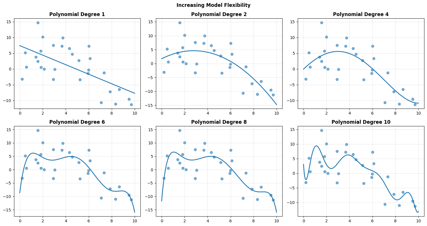
As degree increases:

• The curve bends more easily

• Training error typically decreases

• Sensitivity to noise increases

Low flexibility leads to underfitting. Excessive flexibility leads to overfitting.

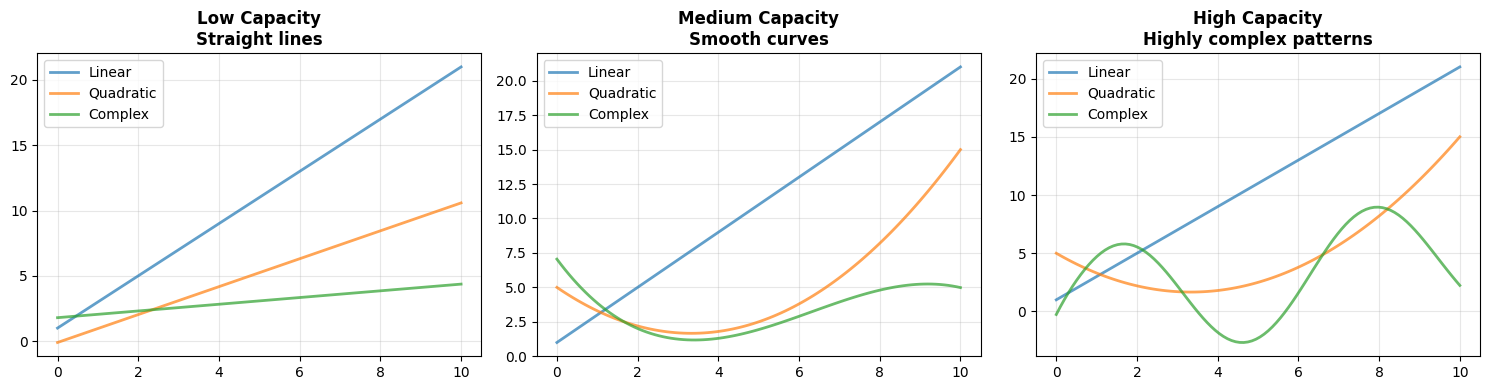
Model Capacity

Capacity refers to the range of functions a model can represent, regardless of whether it actually learns them.

Think of capacity as the model’s vocabulary of patterns.

• Low capacity → can express only simple relationships

• Medium capacity → can capture moderate curvature

• High capacity → can represent highly complex patterns

Show code cell source

Hide code cell source

fig, axes = plt.subplots(1, 3, figsize=(15, 4))

capacities = [
    ("Low Capacity", 1, "Straight lines"),
    ("Medium Capacity", 3, "Smooth curves"),
    ("High Capacity", 9, "Highly complex patterns")
]

patterns = [
    ("Linear", np.random.uniform(0, 10, 30), lambda x: 2*x + 1),
    ("Quadratic", np.random.uniform(0, 10, 30), lambda x: 0.3*x**2 - 2*x + 5),
    ("Complex", np.random.uniform(0, 10, 30), lambda x: 5*np.sin(x) + 0.5*x)
]

for ax, (cap_name, degree, description) in zip(axes, capacities):
    X_test = np.linspace(0, 10, 100).reshape(-1, 1)

    for pattern_name, X_data, pattern_func in patterns:
        X_sorted = np.sort(X_data).reshape(-1, 1)
        y_true = pattern_func(X_sorted.ravel())

        model = make_pipeline(PolynomialFeatures(degree), LinearRegression())
        model.fit(X_sorted, y_true)
        y_pred = model.predict(X_test)

        ax.plot(X_test, y_pred, label=pattern_name, linewidth=2, alpha=0.7)

    ax.set_title(f'{cap_name}\n{description}', fontweight='bold')
    ax.legend()
    ax.grid(True, alpha=0.3)

plt.tight_layout()
plt.show()

Capacity determines what a model can represent, not necessarily what it will learn.

• Low capacity models struggle with complex structure

• High capacity models can approximate almost any function

• Very high capacity models can also memorize noise

Increasing complexity increases expressive power, but also increases the risk of overfitting. The goal is not to maximize complexity, but to match it appropriately to the underlying structure of the data.

6.1.4.3. Simple Models

When we begin modeling, we often start with something deliberately modest. A simple model makes strong assumptions about how the world works. In return, it offers clarity, stability, and interpretability.

A linear regression model is the canonical example. It assumes that the relationship between input and output can be described by a straight line.

from sklearn.linear_model import Ridge
from sklearn.linear_model import LinearRegression

# Generate data
np.random.seed(42)
X_simple = np.random.uniform(0, 10, 50).reshape(-1, 1)
y_simple = 3*X_simple.ravel() + 2 + np.random.normal(0, 2, 50)

# Train simple model
model_simple = LinearRegression()
model_simple.fit(X_simple, y_simple)

LinearRegression()

In a Jupyter environment, please rerun this cell to show the HTML representation or trust the notebook.
On GitHub, the HTML representation is unable to render, please try loading this page with nbviewer.org.

The fitted model is:

[ y = 2.96 * X + 2.19 ]

It contains only two parameters: a slope and an intercept. Its assumption is explicit: the relationship between (X) and (y) is linear.

Show code cell source

Hide code cell source

plt.figure(figsize=(10, 5))
plt.scatter(X_simple, y_simple, s=60, alpha=0.6, label='Data')
X_plot = np.linspace(0, 10, 100).reshape(-1, 1)
y_plot = model_simple.predict(X_plot)
plt.plot(X_plot, y_plot, linewidth=2, label='Linear Model')
plt.xlabel('X')
plt.ylabel('y')
plt.title('A Simple Model: Smooth and Stable')
plt.legend()
plt.grid(True, alpha=0.3)
plt.tight_layout()
plt.show()

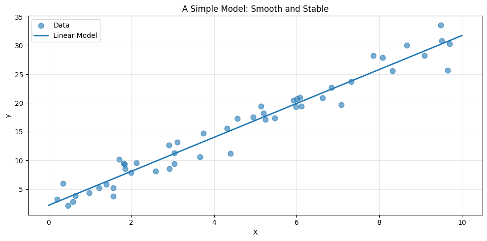
Notice the smoothness of the prediction. The model does not chase individual fluctuations in the data. It captures the overall trend and ignores the noise.

Simple models typically:

• Have few parameters

• Impose strong structural assumptions

• Train quickly

• Are easy to interpret

• Resist overfitting when data is limited

Their limitation is equally clear. If the true pattern bends or curves, a straight line cannot capture it.

6.1.4.4. Complex Models

At the other end of the spectrum are flexible, high capacity models. These models make fewer assumptions about structure and allow the data to shape the prediction.

A random forest is one such model.

from sklearn.ensemble import RandomForestRegressor

model_complex = RandomForestRegressor(
    n_estimators=100,
    max_depth=10,
    random_state=42
)
model_complex.fit(X_simple, y_simple)

RandomForestRegressor(max_depth=10, random_state=42)

In a Jupyter environment, please rerun this cell to show the HTML representation or trust the notebook.
On GitHub, the HTML representation is unable to render, please try loading this page with nbviewer.org.

A random forest is an ensemble of decision trees. Each tree partitions the input space into regions and assigns predictions within those regions. With many trees combined, the model becomes highly expressive.

Show code cell source

Hide code cell source

plt.figure(figsize=(10, 5))
plt.scatter(X_simple, y_simple, s=60, alpha=0.6, label='Data')

y_plot_complex = model_complex.predict(X_plot)
plt.plot(X_plot, y_plot_complex, linewidth=2, label='Random Forest')
plt.plot(X_plot, y_plot, linestyle='--', linewidth=2, alpha=0.6, label='Linear Model')

plt.xlabel('X')
plt.ylabel('y')
plt.title('A Complex Model: Flexible and Adaptive')
plt.legend()
plt.grid(True, alpha=0.3)
plt.tight_layout()
plt.show()

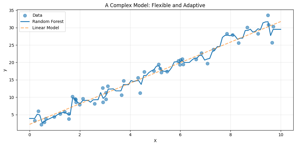
Compared to the linear model, the forest adapts more closely to local variations. It can bend, flatten, and shift depending on the data in each region.

Complex models generally:

• Contain many effective parameters

• Make weaker assumptions

• Capture nonlinear structure

• Require more computation

• Are harder to interpret

They are powerful, but power comes with risk. With limited data, flexibility can turn into overfitting.

6.1.4.5. The Complexity Spectrum

Models do not fall into neat categories. They lie along a continuum, from rigid to highly expressive.

Show code cell source

Hide code cell source

models_spectrum = [
    ("Linear\nRegression", 1),
    ("Logistic\nRegression", 2),
    ("Naive\nBayes", 2.5),
    ("SVM\n(Linear)", 3),
    ("Decision\nTree (small)", 4),
    ("k-NN\n", 5),
    ("SVM\n(RBF)", 6),
    ("Random\nForest", 7),
    ("Gradient\nBoosting", 8),
    ("Deep\nNeural Net", 9.5)
]

fig, ax = plt.subplots(figsize=(14, 3))

for name, complexity in models_spectrum:
    ax.scatter(complexity, 0, s=1000, alpha=0.8)
    ax.text(complexity, -0.25, name, ha='center', fontsize=9)

ax.set_xlim(0, 10)
ax.set_ylim(-0.5, 0.6)
ax.axis('off')
ax.set_title('The Model Complexity Spectrum')

plt.tight_layout()
plt.show()

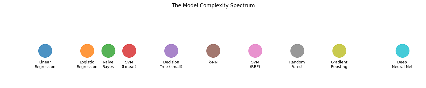
Where a model should sit on this spectrum depends on:

• The amount of data available

• The true complexity of the underlying pattern

• The need for interpretability

• Computational constraints

There is no universally best level of complexity. There is only an appropriate match between model and problem.

---

6.1.4.6. The Goldilocks Principle

To understand this trade off, consider a dataset generated from a quadratic relationship.

Show code cell source

Hide code cell source

np.random.seed(42)
X_gold = np.sort(np.random.uniform(0, 10, 40)).reshape(-1, 1)
true_function = lambda x: 5 + 3*x - 0.3*x**2
y_gold = true_function(X_gold.ravel()) + np.random.normal(0, 2, 40)

X_test = np.sort(np.random.uniform(0, 10, 20)).reshape(-1, 1)
y_test = true_function(X_test.ravel()) + np.random.normal(0, 2, 20)

degrees = [1, 2, 9]
titles = ["Too Simple\n(Underfitting)", "Just Right", "Too Complex\n(Overfitting)"]

fig, axes = plt.subplots(1, 3, figsize=(15, 4))

for ax, degree, title in zip(axes, degrees, titles):
    model = make_pipeline(PolynomialFeatures(degree), LinearRegression())
    model.fit(X_gold, y_gold)

    train_score = model.score(X_gold, y_gold)
    test_score = model.score(X_test, y_test)

    X_plot = np.linspace(0, 10, 200).reshape(-1, 1)
    y_plot = model.predict(X_plot)
    y_true_plot = true_function(X_plot.ravel())

    ax.scatter(X_gold, y_gold, color='blue', s=50, alpha=0.6, label='Train data')
    ax.scatter(X_test, y_test, color='green', s=80, marker='s', alpha=0.7, label='Test data')
    ax.plot(X_plot, y_true_plot, 'k--', linewidth=2, alpha=0.5, label='True function')
    ax.plot(X_plot, y_plot, 'r-', linewidth=2, label='Model')

    ax.set_title(f'{title}\nTrain R²: {train_score:.2f} | Test R²: {test_score:.2f}')
    ax.grid(True, alpha=0.3)

plt.tight_layout()
plt.show()

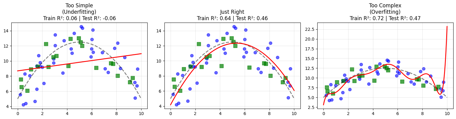
Three regimes emerge:

• A degree 1 model underfits. It misses the curvature entirely.

• A degree 2 model captures the true structure.

• A high degree model fits the noise, achieving near perfect training performance but worse test performance.

This is the Goldilocks principle of modeling. Too simple misses structure. Too complex memorizes noise. The goal is a model that is just complex enough to capture the true signal.

---

6.1.4.7. Complexity and Performance

If we increase complexity systematically, a pattern appears.

from sklearn.model_selection import cross_val_score

degrees = range(1, 16)
train_scores = []
test_scores = []

for degree in degrees:
    model = make_pipeline(PolynomialFeatures(degree), LinearRegression())
    model.fit(X_gold, y_gold)

    train_scores.append(model.score(X_gold, y_gold))
    test_scores.append(model.score(X_test, y_test))

Show code cell source

Hide code cell source

plt.figure(figsize=(12, 6))
plt.plot(degrees, train_scores, 'o-', label='Training Score')
plt.plot(degrees, test_scores, 's-', label='Test Score')

plt.xlabel('Model Complexity (Polynomial Degree)')
plt.ylabel('R² Score')
plt.title('Complexity vs Performance')
plt.legend()
plt.grid(True, alpha=0.3)
plt.tight_layout()
plt.show()

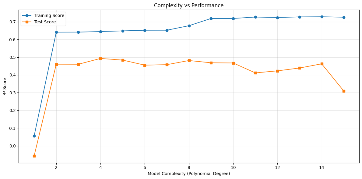
Two consistent observations arise:

1. Training performance improves monotonically with complexity.

2. Test performance improves up to a point, then declines.

The optimal model is located at the peak of the test curve. Beyond that point, additional flexibility improves the fit to training data but harms generalization.

---

6.1.4.8. Choosing the Right Complexity

In practice:

• Begin with the simplest reasonable model.

• Increase complexity only when evidence demands it.

• Use validation data to monitor generalization.

• Watch the gap between training and test performance.

• Remember that more data can justify more complex models.

Modeling is not about maximizing flexibility. It is about aligning model capacity with the true structure of the problem.