6.3.1.1. K-Means Clustering#
K-Means is the most widely used clustering algorithm and the natural starting point for any grouping task. The core idea is simple: represent each cluster by its centroid (the mean of its members) and assign every point to the nearest centroid.
Because it relies only on distances to a small set of centroids, K-Means is:
Fast — linear time per iteration; scales to millions of points.
Interpretable — each cluster has a concrete prototype you can inspect.
A strong baseline — always run K-Means first to get a reference partition.
The Intuition#
Imagine scattering k seed points randomly across your data. You then carry out two alternating steps:
Assign — each data point joins the cluster of the nearest seed.
Update — each seed moves to the mean position of its current members.
Repeat until the seeds stop moving. The seeds have “converged” to the cluster centroids. This is Lloyd’s algorithm.
The key insight is that each step can only lower the total within-cluster distance — so the algorithm is guaranteed to converge, though not necessarily to the global optimum.
The Math#
Objective (Within-Cluster Sum of Squares — WCSS):
where \(C_j\) is the set of points in cluster \(j\) and \(\boldsymbol{\mu}_j\) is its centroid.
Assignment step — for each point assign it to the nearest centroid:
Update step — recompute each centroid as the arithmetic mean:
Both steps strictly decrease \(J\) (or leave it unchanged at convergence). Because \(J\) is bounded below by zero, the algorithm must eventually stop.
Choosing k — the Elbow Method:
Plot WCSS against the number of clusters. WCSS falls steeply at first, then flattens. The “elbow” is the point of diminishing returns and suggests a sensible \(k\).
In scikit-learn#
from sklearn.cluster import KMeans
from sklearn.preprocessing import StandardScaler

scaler  = StandardScaler()
X_sc    = scaler.fit_transform(X)

km = KMeans(n_clusters=3, init='k-means++', n_init=10, random_state=42)
km.fit(X_sc)
labels     = km.labels_          # cluster assignment for each point
centroids  = km.cluster_centers_ # centroid coordinates (scaled space)
inertia    = km.inertia_          # WCSS
Key parameters:
Parameter |
Meaning |
|---|---|
|
Number of clusters k |
|
|
|
Number of restarts; best result is kept |
|
Maximum iterations per run |
Tip
Always standardise features before running K-Means. Euclidean distance is sensitive to scale: a feature measured in thousands will dominate a feature measured in fractions.
Example#
Choosing k with the Elbow Method#
inertias   = []
sil_scores = []
k_range    = range(2, 10)

for k in k_range:
    km = KMeans(n_clusters=k, init='k-means++', n_init=10, random_state=42)
    km.fit(X_sc)
    inertias.append(km.inertia_)
    sil_scores.append(silhouette_score(X_sc, km.labels_))

fig, axes = plt.subplots(1, 2, figsize=(12, 4))

axes[0].plot(k_range, inertias, marker='o', color='steelblue', linewidth=2)
axes[0].axvline(3, color='tomato', linestyle='--', linewidth=1.5, label='k = 3 (elbow)')
axes[0].set_xlabel('Number of clusters k', fontsize=12)
axes[0].set_ylabel('WCSS (Inertia)', fontsize=12)
axes[0].set_title('Elbow Method', fontsize=13, fontweight='bold')
axes[0].legend()
axes[0].grid(True, alpha=0.3)

axes[1].plot(k_range, sil_scores, marker='s', color='seagreen', linewidth=2)
axes[1].axvline(3, color='tomato', linestyle='--', linewidth=1.5, label='k = 3 (best sil)')
axes[1].set_xlabel('Number of clusters k', fontsize=12)
axes[1].set_ylabel('Silhouette Score', fontsize=12)
axes[1].set_title('Silhouette Score vs k', fontsize=13, fontweight='bold')
axes[1].legend()
axes[1].grid(True, alpha=0.3)

plt.suptitle('Wine Dataset — Choosing the Number of Clusters', fontsize=14, fontweight='bold')
plt.tight_layout()
plt.show()
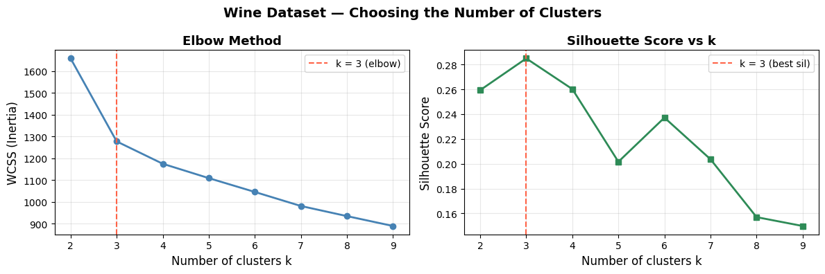
Both diagnostics point to \(k = 3\), which matches the three wine cultivars in the dataset — a good sign.
Fitting the Final Model#
from sklearn.decomposition import PCA

km_final = KMeans(n_clusters=3, init='k-means++', n_init=10, random_state=42)
km_final.fit(X_sc)

# Project to 2D for visualisation
pca = PCA(n_components=2)
X_2d     = pca.fit_transform(X_sc)
centers_2d = pca.transform(km_final.cluster_centers_)

fig, axes = plt.subplots(1, 2, figsize=(13, 5))

titles    = ['K-Means Clusters (predicted)', 'True Wine Cultivars']
label_sets = [km_final.labels_, y]
cmaps     = ['tab10', 'tab10']

for ax, labels_plot, title in zip(axes, label_sets, titles):
    sc = ax.scatter(X_2d[:, 0], X_2d[:, 1], c=labels_plot,
                    cmap='tab10', alpha=0.7, edgecolors='k', linewidths=0.3, s=50)
    ax.set_xlabel('PC 1', fontsize=11)
    ax.set_ylabel('PC 2', fontsize=11)
    ax.set_title(title, fontsize=12, fontweight='bold')
    ax.grid(True, alpha=0.3)

# mark centroids on the prediction plot
axes[0].scatter(centers_2d[:, 0], centers_2d[:, 1],
                marker='X', s=250, c='black', zorder=5, label='Centroids')
axes[0].legend()

plt.suptitle('K-Means on Wine Dataset (2-D PCA projection)', fontsize=14, fontweight='bold')
plt.tight_layout()
plt.show()

sil = silhouette_score(X_sc, km_final.labels_)
print(f"Silhouette Score (k=3): {sil:.3f}")
Silhouette Score (k=3): 0.285
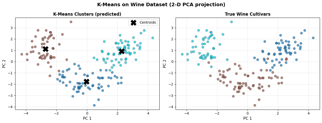
K-Means recovers the three cultivar groups well. The discovered clusters align closely with the true labels, confirming that wine chemical composition is naturally partitioned into three groups.
Strengths and Weaknesses#
Strengths |
Fast and scalable; simple to implement and understand; works well with spherical, similarly-sized clusters |
Weaknesses |
Requires k in advance; sensitive to scale and outliers; assumes convex clusters; may converge to local optimum |
Note
K-Means assumes clusters are convex and similarly sized. If your data has elongated, ring-shaped, or very different-sized clusters, consider DBSCAN or hierarchical clustering instead.