Principal Component Analysis (PCA)

6.3.2.1. Principal Component Analysis (PCA)#

High-dimensional data is hard to understand, slow to process, and often riddled with redundancy. PCA is the most widely used method for addressing all three issues at once.

The core idea is elegant: find the directions in feature space along which the data varies the most, and project everything onto those directions. The first direction (principal component 1) captures maximum variance; the second captures as much of the remaining variance as possible, and so on. Keeping only the top \(k\) components gives a compact, information-rich summary of the original data.

Because PCA is a deterministic, linear method with a closed-form solution, it is:

Reproducible — run it twice, get the same answer.
Fast — computable via standard linear algebra in \(O(np^2)\) time.
Interpretable — each component is an explicit linear combination of the original features.
A pipeline building block — reduce noise and correlation before handing data to a supervised model.

The Math#

Step 1 — Centre the data:

\[\mathbf{X}_c = \mathbf{X} - \bar{\mathbf{x}}\]

Step 2 — Compute the covariance matrix:

\[\mathbf{C} = \frac{1}{n-1} \mathbf{X}_c^\top \mathbf{X}_c \in \mathbb{R}^{p \times p}\]

Step 3 — Eigendecomposition:

\[\mathbf{C} = \mathbf{V} \boldsymbol{\Lambda} \mathbf{V}^\top\]

where the columns of \(\mathbf{V}\) are the eigenvectors (principal component directions) and the diagonal entries of \(\boldsymbol{\Lambda}\) are the eigenvalues \(\lambda_1 \geq \lambda_2 \geq \cdots \geq \lambda_p\).

Step 4 — Project:

\[\mathbf{Z} = \mathbf{X}_c \mathbf{V}_k\]

where \(\mathbf{V}_k\) contains only the top \(k\) eigenvectors. The eigenvalue \(\lambda_j\) is exactly the variance explained by component \(j\).

Variance explained by component \(j\):

\[\text{VE}_j = \frac{\lambda_j}{\sum_{i=1}^{p} \lambda_i}\]

In scikit-learn#

from sklearn.decomposition import PCA
from sklearn.preprocessing import StandardScaler

scaler = StandardScaler()
X_sc   = scaler.fit_transform(X)

pca    = PCA(n_components=2)
X_pca  = pca.fit_transform(X_sc)

Key attributes after fitting:

Attribute	Meaning
`pca.explained_variance_ratio_`	Fraction of variance captured by each component
`pca.components_`	The principal component directions (rows)
`pca.explained_variance_`	Raw eigenvalues

Key parameters:

Parameter	Meaning
`n_components`	Number of components to keep (integer) or variance to retain (float, e.g. `0.95`)
`whiten`	Scale components to unit variance (useful before kNN or SVM)

Tip

Always standardise features before PCA. Without standardisation, features with large numerical ranges dominate the first principal component, regardless of their importance.

Example#

How Much Variance Does Each Component Capture?#

pca_full = PCA().fit(X_sc)

cumvar = np.cumsum(pca_full.explained_variance_ratio_)

fig, axes = plt.subplots(1, 2, figsize=(13, 4))

# Scree plot
axes[0].bar(range(1, 21), pca_full.explained_variance_ratio_[:20],
            color='steelblue', edgecolor='black', linewidth=0.5)
axes[0].set_xlabel('Principal Component', fontsize=12)
axes[0].set_ylabel('Variance Explained', fontsize=12)
axes[0].set_title('Scree Plot (top 20 PCs)', fontsize=13, fontweight='bold')
axes[0].grid(True, alpha=0.3, axis='y')

# Cumulative variance
axes[1].plot(cumvar, linewidth=2, color='seagreen')
axes[1].axhline(0.90, color='tomato',  linestyle='--', linewidth=1.5, label='90 % variance')
axes[1].axhline(0.95, color='darkorange', linestyle='--', linewidth=1.5, label='95 % variance')
n90 = np.argmax(cumvar >= 0.90) + 1
n95 = np.argmax(cumvar >= 0.95) + 1
axes[1].axvline(n90, color='tomato',     linestyle=':', linewidth=1)
axes[1].axvline(n95, color='darkorange', linestyle=':', linewidth=1)
axes[1].set_xlabel('Number of Components', fontsize=12)
axes[1].set_ylabel('Cumulative Variance Explained', fontsize=12)
axes[1].set_title('Cumulative Variance', fontsize=13, fontweight='bold')
axes[1].legend(); axes[1].grid(True, alpha=0.3)

plt.suptitle('Digits Dataset (64 features) — PCA Variance Analysis', fontsize=14, fontweight='bold')
plt.tight_layout()
plt.show()

print(f"Components for 90 % variance: {n90}")
print(f"Components for 95 % variance: {n95}")
print(f"Original dimensionality: {X_sc.shape[1]}")

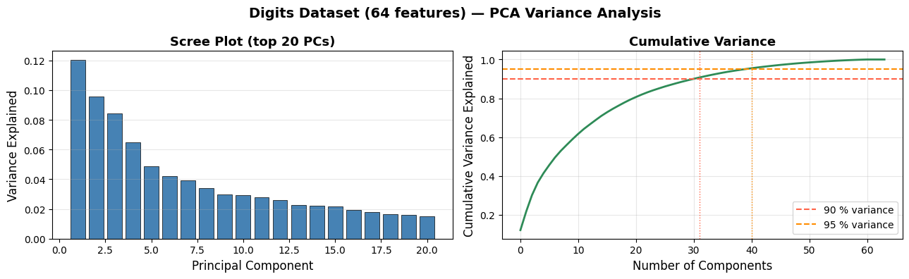
../../../../_images/0125dec86986a2a81742c82e8f610df2b460eb08aafcfbeaab803d543bb8a467.png

Components for 90 % variance: 31
Components for 95 % variance: 40
Original dimensionality: 64

Retaining 41 components (out of 64) already captures 95 % of the variance — roughly a 35 % compression with almost no information loss.

PCA for Visualisation#

Projecting the 64-dimensional digit images onto the first two principal components gives us a 2-D map of the dataset. Despite the extreme compression, distinct clusters emerge for each digit class.

pca2 = PCA(n_components=2)
X_2d = pca2.fit_transform(X_sc)

fig, ax = plt.subplots(figsize=(10, 7))
scatter = ax.scatter(X_2d[:, 0], X_2d[:, 1],
                     c=y, cmap='tab10', alpha=0.6,
                     edgecolors='k', linewidths=0.2, s=25)
cbar = plt.colorbar(scatter, ax=ax, ticks=range(10))
cbar.set_label('Digit class', fontsize=11)
ax.set_xlabel(f'PC 1  ({pca2.explained_variance_ratio_[0]:.1%} variance)', fontsize=12)
ax.set_ylabel(f'PC 2  ({pca2.explained_variance_ratio_[1]:.1%} variance)', fontsize=12)
ax.set_title('Digits Dataset — 2-D PCA Projection', fontsize=14, fontweight='bold')
ax.grid(True, alpha=0.3)
plt.tight_layout()
plt.show()

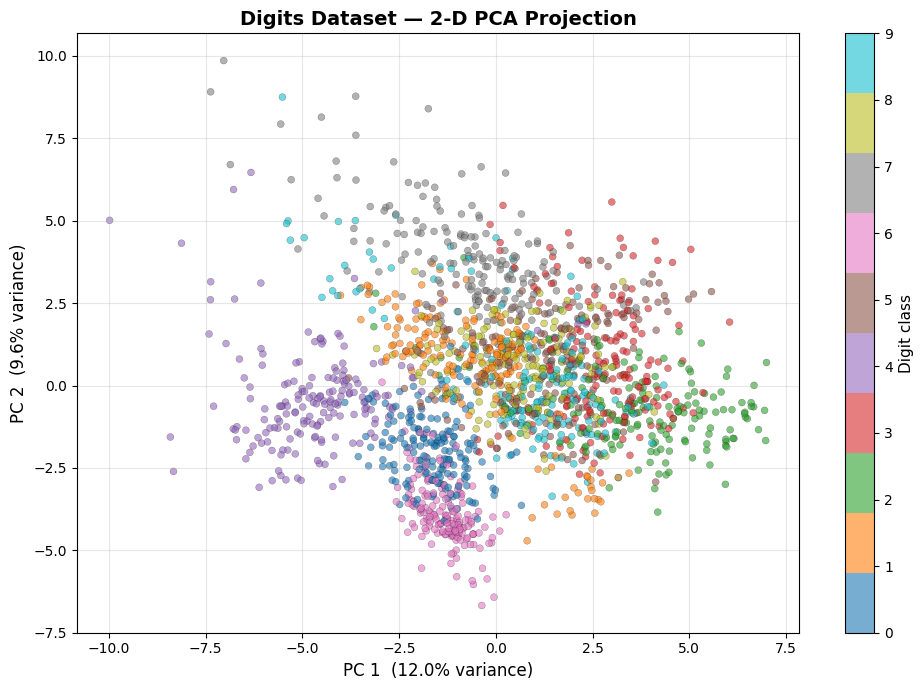
../../../../_images/5058bb48c62753b7fd896c17f09582940c2eeeaf6b5049af646fa6fb706781a4.png

Even with only two components, digits 0 (purple) and 1 (blue) already appear well-separated. The central clump of overlapping classes is where PCA — a linear method — hits its limits; t-SNE and UMAP: Uniform Manifold Approximation and Projection will resolve these clusters far more cleanly.

PCA as a Pre-processing Step#

from sklearn.linear_model import LogisticRegression
from sklearn.pipeline import Pipeline
from sklearn.model_selection import cross_val_score

results = {}
for n in [2, 10, 20, 41, 64]:
    pipe = Pipeline([
        ('pca', PCA(n_components=min(n, 64))),
        ('clf', LogisticRegression(max_iter=1000, random_state=42)),
    ])
    cv_acc = cross_val_score(pipe, X_sc, y, cv=5, scoring='accuracy').mean()
    results[n] = cv_acc

fig, ax = plt.subplots(figsize=(9, 4))
ax.plot(list(results.keys()), list(results.values()), marker='o', linewidth=2, color='steelblue')
ax.axhline(results[64], color='grey', linestyle='--', linewidth=1.2, label='No reduction (64 dims)')
ax.set_xlabel('PCA components retained', fontsize=12)
ax.set_ylabel('5-fold CV Accuracy', fontsize=12)
ax.set_title('Logistic Regression Accuracy vs PCA Compression', fontsize=13, fontweight='bold')
ax.legend(); ax.grid(True, alpha=0.3)
plt.tight_layout()
plt.show()

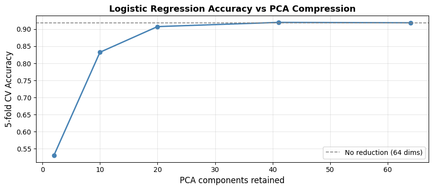
../../../../_images/1e97517d319c22a59e98256b702dcfdafbf35c5656ba108428d2c3485ed51236.png

Accuracy is nearly the same at 41 components as at 64, confirming that the discarded components mostly carry noise. Dropping all the way to 10 components still yields competitive accuracy at a fraction of the computational cost.

Strengths and Weaknesses#


Strengths	Deterministic and reproducible; fast closed-form solution; removes correlated features and noise; interpretable via loadings
Weaknesses	Only captures linear structure; components can be hard to interpret intuitively; sensitive to feature scale (must standardise); cannot be used for new data without refitting to same PC space