6.1.1. What Does It Mean to Model?#
Here, let’s explore what a model actually is and why models are central to machine learning. You might have heard terms like “machine learning model” or “predictive model” without fully understanding what they mean. Let’s build that intuition from the ground up.
6.1.1.1. Why We Need Models#
Imagine you’re running an online store and want to predict which products a customer might buy based on their browsing history. Or perhaps you’re a doctor trying to diagnose a disease based on symptoms and test results. In both cases, you’re trying to find patterns in data to make predictions or decisions.
Traditionally, we might approach these problems using explicit rules:
Start with a base price of $100,000
Add $100 for every square foot
Add $15,000 for each bedroom
If the house is downtown, multiply the price by 1.5
If the house is in the suburbs, multiply the price by 1.2
Example: For a 1,500 square foot, 3-bedroom house in downtown:
Base: $100,000
Size: 1,500 × \(100 = \)150,000
Bedrooms: 3 × \(15,000 = \)45,000
Subtotal: $295,000
Downtown multiplier: $295,000 × 1.5 = $442,500
This approach has serious limitations:
Hard to capture complex patterns - Real relationships are rarely this simple
Requires domain expertise - You need to know all the rules upfront
Doesn’t adapt - Rules don’t improve with more data
Misses hidden patterns - Human experts can’t see every pattern in the data
This is where machine learning models come in. Instead of writing explicit rules, we let the model learn patterns from data.
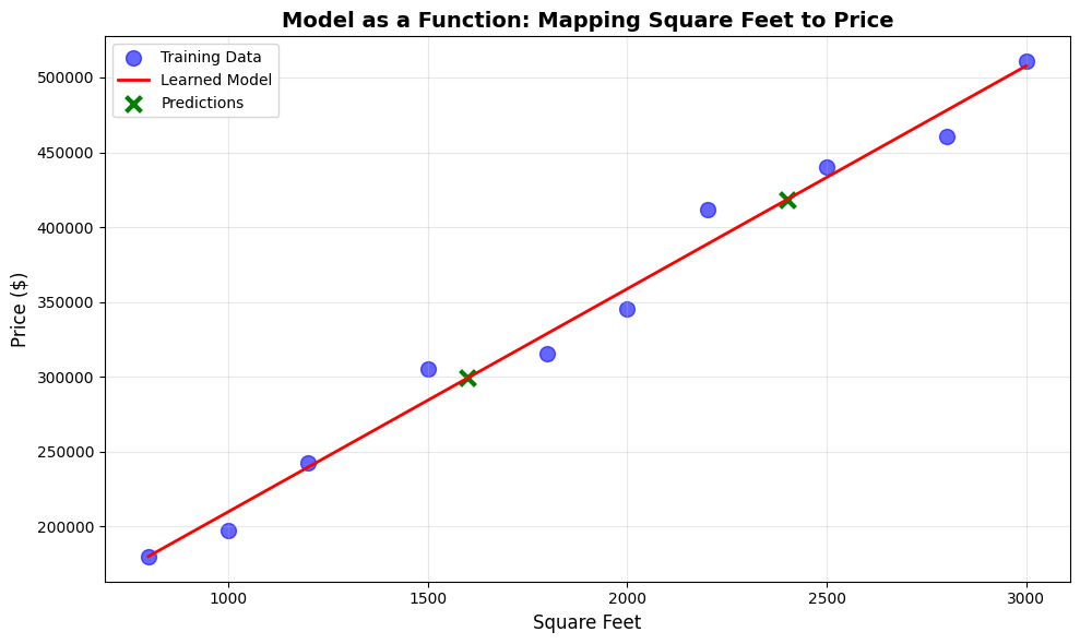
6.1.1.2. Models as Functions: The Core Concept#
At its heart, a model is simply a mathematical function that maps inputs to outputs:
Where:
x represents your input features (square feet, bedrooms, location)
y represents your target output (house price)
f is the model that learns the mapping
The key difference from traditional programming:
Traditional programming: You design the function f explicitly
Machine learning: The algorithm discovers f by learning from examples
Let’s see a concrete example. Don’t worry about understanding all the code details yet, we’re just demonstrating how a model works.
import numpy as np
import matplotlib.pyplot as plt
from sklearn.linear_model import LinearRegression

# Generate synthetic data
np.random.seed(42)
square_feet = np.array([800, 1000, 1200, 1500, 1800, 2000, 2200, 2500, 2800, 3000])
prices = 50000 + 150 * square_feet + np.random.normal(0, 20000, size=10)

X = square_feet.reshape(-1, 1)
y = prices

# Train the model
model = LinearRegression()
model.fit(X, y)

# Make predictions
new_house_sqft = np.array([[1600], [2400]])
predictions = model.predict(new_house_sqft)
The model learned the function: price = 61050 + 149 × square_feet
For a 1600 sq ft house, it predicts $299,272, and for a 2400 sq ft house, $418,384.
What happened:
We gave the model examples (square feet and prices)
The model discovered the pattern automatically
Now it can predict prices for houses it’s never seen
This is learning from data.
6.1.1.3. The Machine Learning Workflow#
Every machine learning project follows this general workflow:
1. Collect Data#
You need examples showing both inputs (features) and outputs (target values for supervised learning).
2. Train the Model#
The model analyzes the data to discover patterns. This process is called training or fitting.
model.fit(X_train, y_train) # Model learns patterns
3. Make Predictions#
Once trained, the model can make predictions on new, unseen data. This is called inference or prediction.
predictions = model.predict(X_new) # Model applies learned patterns
4. Evaluate Performance#
Check how well the model performs on data it hasn’t seen before.
score = model.score(X_test, y_test) # Measure accuracy
Let’s see this complete workflow:
from sklearn.model_selection import train_test_split
from sklearn.metrics import mean_absolute_error, r2_score

# Generate synthetic data
np.random.seed(42)
n_samples = 100
square_feet = np.random.uniform(800, 3500, n_samples)
prices = 50000 + 150 * square_feet + np.random.normal(0, 30000, size=n_samples)

X = square_feet.reshape(-1, 1)
y = prices

# Split data into train and test
X_train, X_test, y_train, y_test = train_test_split(X, y, test_size=0.2, random_state=42)

# Train model
model = LinearRegression()
model.fit(X_train, y_train)

# Make predictions
y_pred = model.predict(X_test)

# Evaluate model
mae = mean_absolute_error(y_test, y_pred)
r2 = r2_score(y_test, y_pred)
Model Performance:
Mean Absolute Error: $ 17,740
R² Score: 0.961
This means predictions are off by $ 17,740 on average.
6.1.1.4. Parameters vs. Hyperparameters#
When working with models, you’ll encounter two types of values:
Parameters#
Values that the model learns from the data during training.
In our linear model, the parameters are:
Intercept: The baseline price
Coefficient: How much price increases per square foot
These are discovered automatically by the learning algorithm, giving us:
Intercept: $57,855
Coefficient: $145.54 per sq ft
Hyperparameters#
These are values that you set before training to control how the model learns.
Examples:
The type of model (linear, tree, neural network)
Complexity settings (tree depth, number of layers)
Learning rate (how fast the model adjusts)
# Hyperparameters (you choose these)
from sklearn.tree import DecisionTreeRegressor

model = DecisionTreeRegressor(
    max_depth=5,           # Hyperparameter: How deep the tree can grow
    min_samples_split=10   # Hyperparameter: Minimum samples to split
)
Key distinction:
Parameters: The model learns these (weights, coefficients)
Hyperparameters: You set these (model architecture, training settings)
6.1.1.5. Types of Models#
Models can be broadly categorized by how they represent patterns:
Parametric Models#
Have a fixed form with a specific number of parameters.
Examples:
Linear Regression: y = mx + b (2 parameters: m, b)
Logistic Regression
Neural Networks (fixed architecture)
Advantages:
Fast to train
Easy to interpret
Work well with less data
Disadvantages:
Strong assumptions about data shape
Limited flexibility
from sklearn.linear_model import LinearRegression

# Train model
model_parametric = LinearRegression()
model_parametric.fit(X_train, y_train)
LinearRegression()In a Jupyter environment, please rerun this cell to show the HTML representation or trust the notebook.
On GitHub, the HTML representation is unable to render, please try loading this page with nbviewer.org.
Parameters
| fit_intercept | True | |
| copy_X | True | |
| tol | 1e-06 | |
| n_jobs | None | |
| positive | False |
This model will always have the form: y = mx + b. No matter how much data we give it, it’s constrained to a line. For our example, the model is: 145.5x + 57855.0 with just 2 parameters (slope and intercept).
Non-Parametric Models#
Can grow in complexity with the amount of data.
Examples:
k-Nearest Neighbors
Decision Trees
Kernel SVMs
Advantages:
High flexibility
Few assumptions
Can capture complex patterns
Disadvantages:
Need more data
Can be slower
Risk of overfitting
6.1.1.6. Training vs. Inference#
It’s important to understand these two distinct phases:
Training (Learning Phase)#
The model analyzes examples
Adjusts internal parameters
Discovers patterns
Computationally expensive - can take hours or days
# Training: Model learns (slow)
model.fit(X_train, y_train)  # Could take minutes to hours
Inference (Prediction Phase)#
The model applies learned patterns
Makes predictions on new data
Parameters are frozen - no learning
Fast - milliseconds to seconds
# Inference: Model predicts (fast)
predictions = model.predict(X_new)  # Typically milliseconds
This distinction is crucial:
You train once (or periodically)
You predict many times (potentially millions of times)
6.1.1.7. When to Use Models#
Models are powerful tools, but they are not always the right solution. Use models when:
Patterns are complex – The relationships in the data are too intricate for fixed rules.
Sufficient data is available – You have enough labeled or historical examples to learn from.
Patterns evolve over time – The system can be retrained as new data arrives.
Approximate predictions are acceptable – Some level of error is tolerable.
Avoid using models when:
A simple, deterministic rule can solve the problem reliably.
Data is scarce or low quality.
The system requires near perfect accuracy, such as in safety critical settings.
The cost of incorrect predictions is prohibitively high.