6.2.3.3. Neural Networks#
A single The Perceptron can only learn linearly separable patterns. The moment you add one or more hidden layers between input and output, the network can represent any continuous function - a remarkable result known as the Universal Approximation Theorem.
This architecture - Input Layer → Hidden Layer(s) → Output Layer - is called a Multi-Layer Perceptron (MLP) or feedforward neural network. It is the foundational architecture for all of modern deep learning.
The Core Idea#
Hidden layers transform the input step by step. Each layer learns a new representation of the data - increasingly abstract features built on top of previous ones:
Layer 1: learns simple combinations of raw features
Layer 2: learns combinations of Layer 1’s outputs
Layer L: hands a transformed representation to the output layer
The output layer then applies a task-appropriate activation:
Regression: no activation (linear output)
Binary classification: sigmoid — squashes a single score into a probability in \((0,1)\)
Multi-class: softmax — converts \(K\) raw scores into a probability distribution that sums to 1
The hidden layers nearly always use ReLU (or a variant). The output activation is chosen to match the task — sigmoid for binary, softmax for multi-class, nothing for regression.
The Math#
Forward Pass#
For a network with \(L\) layers, each layer \(\ell\) transforms its input \(\mathbf{a}^{(\ell-1)}\) (where \(\mathbf{a}^{(0)} = \mathbf{x}\)):
where \(W^{(\ell)}\) is the weight matrix for layer \(\ell\) and \(f\) is the activation function applied element-wise.
Output Activations#
Sigmoid (binary classification output)
The sigmoid function takes a single raw score \(z\) and maps it to a probability:
The network outputs one neuron; if \(\sigma(z) \geq 0.5\) the prediction is class 1, otherwise class 0. The loss is binary cross-entropy:
Softmax (multi-class classification output)
For \(K\) classes the network outputs \(K\) neurons with raw scores \(z_1, \ldots, z_K\). Softmax converts them into a probability distribution:
Taking the exponential ensures all outputs are positive; dividing by the sum normalises them. The class with the highest score still gets the largest probability — softmax preserves ordering while making the outputs interpretable as probabilities.
The loss minimised during training is categorical cross-entropy:
Because only the true-class term survives the indicator \(\mathbf{1}[y_i=k]\), this simplifies to: minimise the negative log-probability of the correct class — the higher the probability assigned to the right answer, the lower the loss.
Backpropagation#
Backpropagation is the algorithm that computes \(\nabla_W \mathcal{L}\) efficiently by applying the chain rule backwards through the network:
The gradient at each layer is computed from the gradient at the next layer, passed backwards - hence the name. This is just the chain rule of calculus, applied systematically.
Key hyperparameters:
Hyperparameter |
Role |
|---|---|
|
Number of hidden layers and neurons per layer |
|
|
|
Optimizer - see Optimizers |
|
L2 regularisation strength |
|
Starting step size |
|
Mini-batch size for SGD/Adam |
In scikit-learn#
from sklearn.neural_network import MLPClassifier
from sklearn.preprocessing import StandardScaler
from sklearn.pipeline import Pipeline

mlp = Pipeline([
    ('scaler', StandardScaler()),
    ('mlp', MLPClassifier(
        hidden_layer_sizes=(128, 64),  # two hidden layers
        activation='relu',
        solver='adam',
        alpha=1e-4,                    # L2 regularisation
        learning_rate_init=0.001,
        max_iter=300,
        random_state=42
    ))
])
mlp.fit(X_train, y_train)
Always scale features before training an MLP - gradient descent is highly sensitive to feature magnitudes. A Pipeline ensures the scaler is never accidentally applied to the test set during evaluation.
Example#
from sklearn.neural_network import MLPClassifier

mlp = MLPClassifier(
    hidden_layer_sizes=(128, 64),
    activation='relu',
    solver='adam',
    alpha=1e-4,
    learning_rate_init=0.001,
    max_iter=300,
    random_state=42
)
mlp.fit(X_train_sc, y_train)

train_acc = accuracy_score(y_train, mlp.predict(X_train_sc))
test_acc  = accuracy_score(y_test,  mlp.predict(X_test_sc))
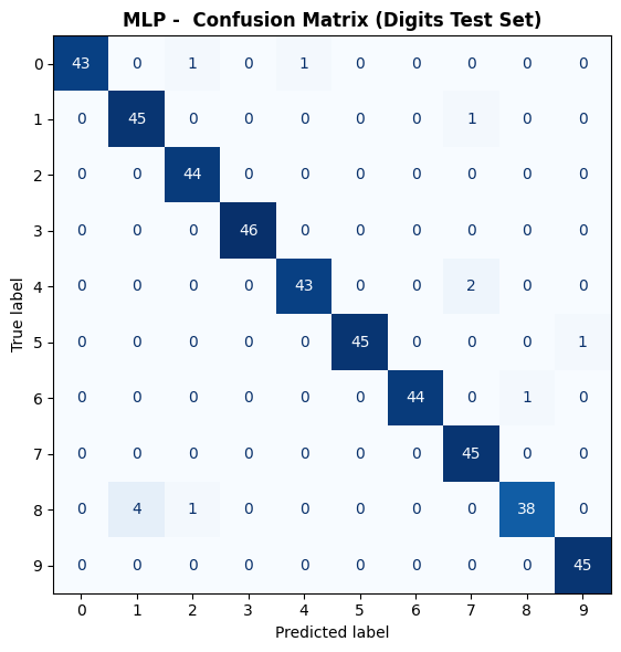
Two hidden layers (128 → 64 → 10) achieves a test accuracy of 0.973, a dramatic improvement over the single-layer The Perceptron. Train accuracy of 1.0 is slightly higher but the gap is small, indicating the L2 regularisation is working.
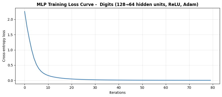
Training Loss Curve#
Monitoring the loss curve is the first thing to do after training. A smooth descent that plateaus is healthy; oscillations suggest the learning rate is too high; a loss that barely moves suggests it is too low.
fig, ax = plt.subplots(figsize=(9, 4))
ax.plot(mlp.loss_curve_, color='steelblue', lw=2)
ax.set_xlabel("Iterations")
ax.set_ylabel("Cross-entropy loss")
ax.set_title("MLP Training Loss Curve -  Digits (128→64 hidden units, ReLU, Adam)",
             fontweight='bold')
ax.grid(True, alpha=0.3)
plt.tight_layout()
plt.show()
Confusion Matrix#
fig, ax = plt.subplots(figsize=(7, 6))
ConfusionMatrixDisplay.from_predictions(
    y_test, mlp.predict(X_test_sc),
    ax=ax, colorbar=False, cmap='Blues'
)
ax.set_title("MLP -  Confusion Matrix (Digits Test Set)", fontweight='bold')
plt.tight_layout()
plt.show()
Effect of Architecture Depth#
Adding hidden layers increases model capacity. Here we compare architectures from no hidden layers (a linear model) up to three hidden layers.
architectures = {
    "No hidden (linear)":   (),
    "1 layer (64)":         (64,),
    "2 layers (128, 64)":   (128, 64),
    "3 layers (256,128,64)":(256, 128, 64),
}

rows = []
for name, size in architectures.items():
    m = MLPClassifier(hidden_layer_sizes=size, activation='relu',
                      solver='adam', alpha=1e-4,
                      max_iter=400, random_state=42)
    m.fit(X_train_sc, y_train)
    rows.append({
        "Architecture":   name,
        "Train Accuracy": round(accuracy_score(y_train, m.predict(X_train_sc)), 3),
        "Test Accuracy":  round(accuracy_score(y_test,  m.predict(X_test_sc)),  3),
        "Iterations":     m.n_iter_,
    })

pd.DataFrame(rows)
/home/runner/work/datasciencethenovel/datasciencethenovel/.venv/lib/python3.13/site-packages/sklearn/neural_network/_multilayer_perceptron.py:781: ConvergenceWarning: Stochastic Optimizer: Maximum iterations (400) reached and the optimization hasn't converged yet.
  warnings.warn(
| Architecture | Train Accuracy | Test Accuracy | Iterations | |
|---|---|---|---|---|
| 0 | No hidden (linear) | 0.997 | 0.964 | 400 |
| 1 | 1 layer (64) | 1.000 | 0.980 | 164 |
| 2 | 2 layers (128, 64) | 1.000 | 0.973 | 80 |
| 3 | 3 layers (256,128,64) | 1.000 | 0.982 | 48 |
Each additional layer captures more abstract features from the digit images, translating into higher accuracy - until the model is large enough that we hit diminishing returns or would need regularisation to prevent overfitting.