6.2.1.3. Regularized Regression

When a linear model has many features - especially when they are correlated or only weakly relevant - Ordinary Least Squares tends to overfit: it assigns large, noisy coefficients to chase training-set variation that does not generalise.

Regularization fixes this by adding a penalty on the magnitude of the coefficients directly to the loss function. The optimiser is now forced to balance fitting the data and keeping the coefficients small. The result is a model that is slightly biased but has much lower variance, and usually generalises much better.

There are three main variants:

Variant	Penalty	Key behaviour
Ridge (L2)	Sum of squared coefficients	Shrinks all coefficients toward zero uniformly; none become exactly zero
Lasso (L1)	Sum of absolute coefficients	Drives some coefficients to exactly zero - automatic feature selection
Elastic Net	Weighted L1 + L2	Combines both: sparse like Lasso, stable with correlated features like Ridge

---

The Math

All three regularized models minimise the same base MSE loss (as in Linear Regression), plus a penalty term controlled by the hyperparameter \(\alpha\).

Ridge (L2)

\[\text{Loss}_{\text{Ridge}} = \frac{1}{n}\sum_{i=1}^{n}(y_i - \hat{y}_i)^2 + \alpha \sum_{j=1}^{p} \beta_j^2\]

The L2 penalty creates a smooth penalty landscape - no direction is treated differently, so all coefficients shrink together. The solution remains unique even when features are correlated.

Lasso (L1)

\[\text{Loss}_{\text{Lasso}} = \frac{1}{n}\sum_{i=1}^{n}(y_i - \hat{y}_i)^2 + \alpha \sum_{j=1}^{p} |\beta_j|\]

The L1 penalty has sharp corners at zero in each dimension. This geometric property means the optimum frequently lands exactly on zero for some coefficients, producing sparse solutions.

Elastic Net

\[\text{Loss}_{\text{EN}} = \text{MSE} + \alpha \left[ \rho \sum_{j=1}^{p}|\beta_j| + \frac{1-\rho}{2} \sum_{j=1}^{p}\beta_j^2 \right]\]

l1_ratio \(\rho = 1\) recovers Lasso; \(\rho = 0\) recovers Ridge. A value like \(0.5\) gives an equal blend.

---

In scikit-learn

from sklearn.linear_model import Ridge, Lasso, ElasticNet

ridge = Ridge(alpha=1.0)
lasso = Lasso(alpha=0.5, max_iter=5000)
enet  = ElasticNet(alpha=0.5, l1_ratio=0.5, max_iter=5000)

Key hyperparameters:

• alpha - regularization strength; higher → stronger shrinkage (use RidgeCV / LassoCV to tune)

• l1_ratio (Elastic Net only) - blend between L1 and L2

---

Example

Show code cell source

Hide code cell source

import numpy as np
import pandas as pd
import matplotlib.pyplot as plt
from myst_nb import glue
from sklearn.linear_model import Ridge, Lasso, ElasticNet
from sklearn.model_selection import train_test_split
from sklearn.metrics import mean_squared_error, r2_score
from sklearn.datasets import make_regression

np.random.seed(42)

X, y = make_regression(n_samples=300, n_features=10, n_informative=6,
                        noise=25, random_state=42)
X_train, X_test, y_train, y_test = train_test_split(
    X, y, test_size=0.25, random_state=42)

def test_stats(model):
    model.fit(X_train, y_train)
    r2   = r2_score(y_test, model.predict(X_test))
    rmse = np.sqrt(mean_squared_error(y_test, model.predict(X_test)))
    return round(r2, 3), round(rmse, 1)

ridge = Ridge(alpha=1.0)
lasso = Lasso(alpha=0.5, max_iter=5000)
enet  = ElasticNet(alpha=0.5, l1_ratio=0.5, max_iter=5000)

ridge_r2, ridge_rmse = test_stats(ridge)
lasso_r2, lasso_rmse = test_stats(lasso)
enet_r2,  enet_rmse  = test_stats(enet)

pd.DataFrame({
    "Model":     ["Ridge (α=1.0)", "Lasso (α=0.5)", "Elastic Net (α=0.5, ρ=0.5)"],
    "Test R²":   [ridge_r2, lasso_r2, enet_r2],
    "Test RMSE": [ridge_rmse, lasso_rmse, enet_rmse],
})

	Model	Test R²	Test RMSE
0	Ridge (α=1.0)	0.978	26.3
1	Lasso (α=0.5)	0.978	26.6
2	Elastic Net (α=0.5, ρ=0.5)	0.924	49.1

Ridge achieves \(R^2\) = 0.978, Lasso 0.978, and Elastic Net 0.924. The dataset has only 6 informative features out of 10, so Lasso’s feature-selection behaviour is particularly relevant here.

Coefficient Paths - How \(\alpha\) Changes the Solution

As \(\alpha\) increases, more regularization is applied and all coefficients shrink. For Lasso, they hit zero one by one:

Show code cell source

Hide code cell source

alphas = np.logspace(-2, 3, 60)
ridge_coefs = np.array([Ridge(alpha=a).fit(X_train, y_train).coef_ for a in alphas])
lasso_coefs = np.array([Lasso(alpha=a, max_iter=10000).fit(X_train, y_train).coef_ for a in alphas])

fig, axes = plt.subplots(1, 2, figsize=(14, 5))
for i in range(X_train.shape[1]):
    axes[0].plot(np.log10(alphas), ridge_coefs[:, i], linewidth=1.4)
    axes[1].plot(np.log10(alphas), lasso_coefs[:, i], linewidth=1.4)

for ax, title in zip(axes, ["Ridge - Coefficient Paths (L2)", "Lasso - Coefficient Paths (L1)"]):
    ax.axhline(0, color="black", linestyle="--", linewidth=0.8)
    ax.set_xlabel("log₁₀(α)", fontsize=12)
    ax.set_ylabel("Coefficient value", fontsize=12)
    ax.set_title(title, fontsize=12, fontweight="bold")
    ax.grid(True, alpha=0.3)

plt.tight_layout()
plt.show()

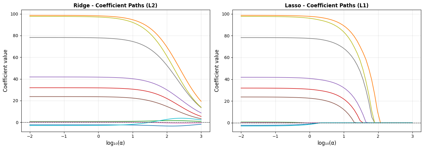
In the Ridge plot, every line smoothly approaches zero but never fully reaches it. In the Lasso plot, lines hit zero and stay there - those are features being excluded from the model entirely.

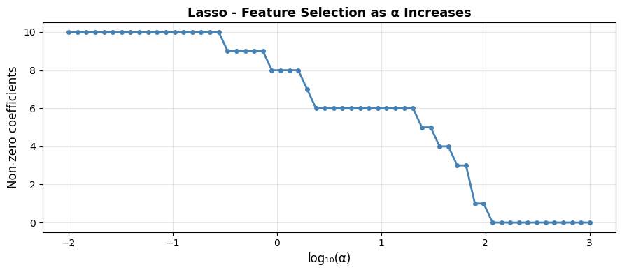
How Many Features Does Lasso Keep?

non_zero_by_alpha = [(np.sum(lasso_coefs[i] != 0)) for i in range(len(alphas))]

plt.figure(figsize=(9, 4))
plt.plot(np.log10(alphas), non_zero_by_alpha, "o-", markersize=4, linewidth=2, color="steelblue")
plt.xlabel("log₁₀(α)", fontsize=12)
plt.ylabel("Non-zero coefficients", fontsize=12)
plt.title("Lasso - Feature Selection as α Increases", fontsize=13, fontweight="bold")
plt.grid(True, alpha=0.3)
plt.tight_layout()
plt.show()

# Count non-zero coefficients in the fitted Lasso (α=0.5)
n_selected = int(np.sum(lasso.coef_ != 0))
glue("lasso-n-selected", n_selected, display=False)

With \(\alpha = 0.5\), Lasso retains 9 of the 10 features, correctly discarding most of the non-informative ones.

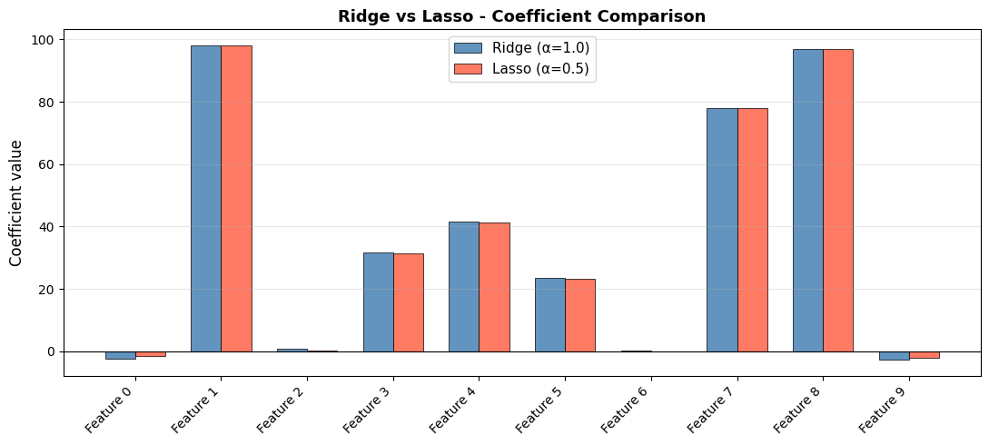
Ridge vs Lasso - Side-by-Side Coefficient Comparison

Show code cell source

Hide code cell source

features = [f"Feature {i}" for i in range(X.shape[1])]
x_pos = np.arange(len(features))
width = 0.35

fig, ax = plt.subplots(figsize=(11, 5))
ax.bar(x_pos - width/2, ridge.coef_, width, label="Ridge (α=1.0)",
       alpha=0.85, edgecolor="black", linewidth=0.6, color="steelblue")
ax.bar(x_pos + width/2, lasso.coef_, width, label="Lasso (α=0.5)",
       alpha=0.85, edgecolor="black", linewidth=0.6, color="tomato")
ax.axhline(0, color="black", linewidth=0.8)
ax.set_xticks(x_pos)
ax.set_xticklabels(features, rotation=45, ha="right", fontsize=10)
ax.set_ylabel("Coefficient value", fontsize=12)
ax.set_title("Ridge vs Lasso - Coefficient Comparison", fontsize=13, fontweight="bold")
ax.legend(fontsize=11)
ax.grid(True, alpha=0.3, axis="y")
plt.tight_layout()
plt.show()

---

Choosing Between Ridge, Lasso, and Elastic Net

Situation	Recommended
Many features, each contributes a little	Ridge - keeps all features, stable
Few features truly matter (sparse signal)	Lasso - zeroes out irrelevant features
Correlated features + you want sparsity	Elastic Net - handles correlations better than pure Lasso
Unsure	Elastic Net - safe default that interpolates between both

Tip

Use RidgeCV, LassoCV, or ElasticNetCV to automatically select alpha via cross-validation instead of guessing.