5.3.1. Data Distribution and Feature Behavior#
Before analyzing relationships between features or comparing data points, it is essential to understand how individual features behave on their own. Data distributions provide a high-level view of how values are spread, how frequently they occur, and what patterns or irregularities may be present.
Many real-world datasets follow common and well-studied distributions. Recognizing these patterns helps us reason about the underlying data-generating process and informs decisions about preprocessing, modeling, and evaluation.
In this section, we examine distributions at the level of single features, consider both numeric and categorical data, and introduce key concepts that describe distribution shape.
5.3.1.1. Univariate Distributions#
Univariate analysis focuses on one feature at a time. It helps identify skewed data, outliers, and the general shape of a feature’s distribution, such as normal, bimodal, or uniform.
For numeric features, histograms are a common visualization tool. They group values into bins and show how frequently values occur within each range.
import sqlite3
import pandas as pd
import matplotlib.pyplot as plt

# Connect to Chinook sample database
conn = sqlite3.connect("../data/chinook.db")

# Load the 'tracks' table into a DataFrame
df_tracks = pd.read_sql_query("SELECT * FROM tracks", conn)
df_tracks.head()
| TrackId | Name | AlbumId | MediaTypeId | GenreId | Composer | Milliseconds | Bytes | UnitPrice | |
|---|---|---|---|---|---|---|---|---|---|
| 0 | 1 | For Those About To Rock (We Salute You) | 1 | 1 | 1 | Angus Young, Malcolm Young, Brian Johnson | 343719 | 11170334 | 0.99 |
| 1 | 2 | Balls to the Wall | 2 | 2 | 1 | None | 342562 | 5510424 | 0.99 |
| 2 | 3 | Fast As a Shark | 3 | 2 | 1 | F. Baltes, S. Kaufman, U. Dirkscneider & W. Ho... | 230619 | 3990994 | 0.99 |
| 3 | 4 | Restless and Wild | 3 | 2 | 1 | F. Baltes, R.A. Smith-Diesel, S. Kaufman, U. D... | 252051 | 4331779 | 0.99 |
| 4 | 5 | Princess of the Dawn | 3 | 2 | 1 | Deaffy & R.A. Smith-Diesel | 375418 | 6290521 | 0.99 |
df_tracks.hist(
    figsize=(12, 10),
    bins=30,
    grid=False,
    edgecolor="black"
)

plt.tight_layout()
plt.show()
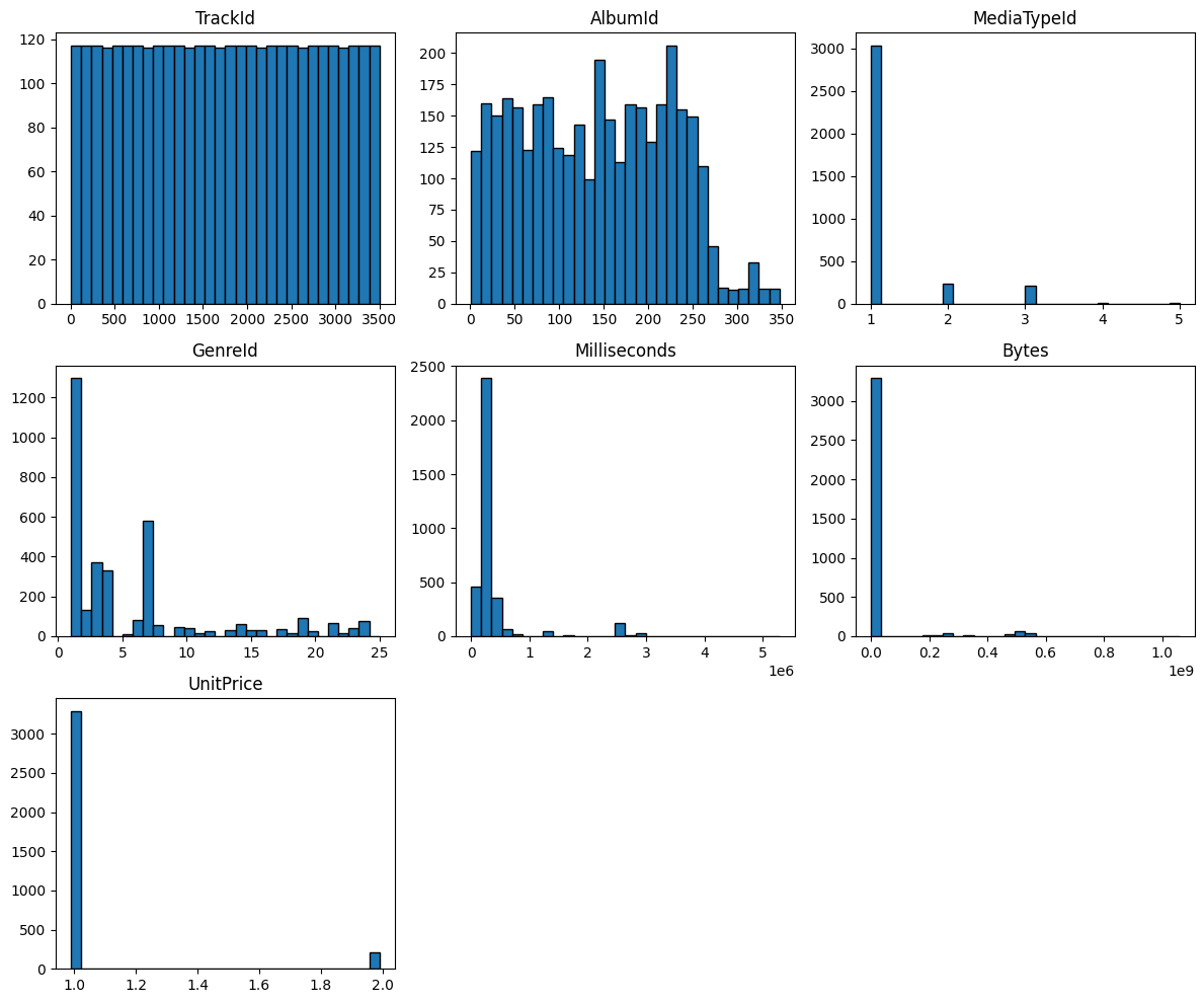
These plots provide a visual summary of features such as Milliseconds, Bytes, and UnitPrice. From these distributions, we can quickly spot skewness, extreme values, and irregular patterns that may require further attention.
5.3.1.2. Categorical Feature Distributions#
Not all features are numeric. Categorical features represent groups or labels rather than quantities. Examples include genre, category, country, or class labels.
For categorical features, distributions are described using frequencies instead of numeric ranges.
Common tools include:
Frequency tables using
value_counts()Bar charts or count plots
Mode as a summary statistic
df_tracks["GenreId"].value_counts()
GenreId
1     1297
7      579
3      374
4      332
2      130
19      93
6       81
24      74
21      64
14      61
8       58
9       48
10      43
23      40
17      35
15      30
16      28
13      28
20      26
12      24
22      17
11      15
18      13
5       12
25       1
Name: count, dtype: int64
Understanding categorical distributions helps identify dominant classes, rare categories, and potential class imbalance, all of which can strongly affect downstream analysis and modeling.
Note
Categorical features should not be treated as numeric unless they have a meaningful ordering and spacing.
5.3.1.3. Empirical and Theoretical Distributions#
The distributions we observe in data are known as empirical distributions, as they are derived directly from collected samples. In contrast, theoretical distributions are mathematical models such as the normal, uniform, or exponential distributions.
In practice, we often compare empirical data to theoretical distributions to assess whether modeling assumptions are reasonable.
Examples of common theoretical distributions include:
Normal distribution for natural variation and measurement noise
Uniform distribution for equally likely outcomes
Exponential distribution for waiting times or lifetimes
Note
Many statistical methods assume an underlying theoretical distribution. Verifying whether this assumption is reasonable begins with empirical distribution analysis.
5.3.1.4. Distribution Shape: Skewness and Kurtosis#
Beyond central tendency and spread, the shape of a distribution provides important information.
Skewness measures the asymmetry of a distribution:
Positive skew indicates a long right tail
Negative skew indicates a long left tail
Zero skew indicates symmetry
Kurtosis measures the heaviness of the tails relative to a normal distribution:
High kurtosis indicates heavy tails and more extreme values
Low kurtosis indicates light tails and fewer outliers
These measures help explain why some features may violate modeling assumptions or require transformation before analysis.
df_tracks.skew(numeric_only=True)
TrackId         0.000000
AlbumId         0.089525
MediaTypeId     3.028186
GenreId         1.560547
Milliseconds    3.951430
Bytes           4.372829
UnitPrice       3.677272
dtype: float64
df_tracks.kurt(numeric_only=True)
TrackId         -1.200000
AlbumId         -1.033178
MediaTypeId      9.602763
GenreId          1.502033
Milliseconds    15.744308
Bytes           19.385956
UnitPrice       11.528913
dtype: float64
5.3.1.5. Why Distribution Analysis Matters#
Understanding feature distributions is a prerequisite for meaningful relationship analysis. Distribution shape influences correlation, distance, and similarity measures, and poorly behaved features can dominate or distort results.
With a clear understanding of how individual features behave, we can now move on to examining how features interact with one another.