6.3.3. Anomaly Detection#
Most data points in a dataset are normal. A small fraction deviate significantly from the rest — these are anomalies (also called outliers). Finding them matters enormously in practice:
Fraudulent credit card transactions among millions of legitimate ones
Faulty sensors in an industrial monitoring system
Rare disease cases in a medical dataset
Unlike clustering or dimensionality reduction, anomaly detection does not group points — it separates the standard from the strange. Because anomalies are rare and often unlabelled, most practical methods are unsupervised.
6.3.3.1. The Core Idea#
The unifying principle across almost all anomaly detection methods is:
Normal points live in dense, well-connected regions of the feature space. Anomalies are isolated, sparse, or geometrically extreme.
Methods differ in how they measure “isolation”:
Method |
How it measures isolation |
|---|---|
Z-Score / IQR |
Distance from the mean / median in standard deviation units |
Isolation Forest |
Anomalies are easier to isolate with random cuts in the feature space |
Local Outlier Factor (LOF) |
A point’s density compared to its neighbours |
6.3.3.2. Isolation Forest#
Isolation Forest is the most practical general-purpose algorithm for tabular data. The core insight is counterintuitive: anomalies are easier to isolate than normal points.
Build a random tree by repeatedly choosing a random feature and a random split value. Normal points, hidden deep in dense regions, require many splits to be isolated. Anomalies, being extreme or sparse, get isolated in just a few splits.
The anomaly score is the average depth across many trees:
where \(h(\mathbf{x})\) is the average isolation path length and \(c(n)\) is the expected path length for a random point in a dataset of size \(n\). A score near 1 indicates a likely anomaly; a score near 0.5 indicates normality.
from sklearn.ensemble import IsolationForest

iso = IsolationForest(contamination=0.05, random_state=42)
iso.fit(X_train)
scores  = iso.decision_function(X_test)  # higher → more normal
labels  = iso.predict(X_test)             # +1 = normal, -1 = anomaly
6.3.3.3. Local Outlier Factor#
LOF compares the local density of a point to the densities of its \(k\) nearest neighbours. If a point is much less dense than its neighbours, it is likely an outlier.
LOF \(\approx 1\) → normal. LOF \(\gg 1\) → anomaly.
LOF is particularly good at detecting contextual anomalies — points that are technically within the range of the data as a whole but are anomalous relative to their local neighbourhood.
from sklearn.neighbors import LocalOutlierFactor

lof    = LocalOutlierFactor(n_neighbors=20, contamination=0.05)
labels = lof.fit_predict(X)   # +1 = normal, -1 = anomaly
scores = -lof.negative_outlier_factor_
6.3.3.4. Example#
iso = IsolationForest(contamination=0.06, random_state=42)
iso_labels = iso.fit_predict(X_sc)

lof = LocalOutlierFactor(n_neighbors=20, contamination=0.06)
lof_labels = lof.fit_predict(X_sc)

fig, axes = plt.subplots(1, 3, figsize=(18, 5))
datasets  = [
    (y_true,     'True Labels'),
    (iso_labels, 'Isolation Forest'),
    (lof_labels, 'Local Outlier Factor'),
]

for ax, (labels, title) in zip(axes, datasets):
    colors = np.where(labels == -1, 'tomato', 'steelblue')
    ax.scatter(X_sc[:, 0], X_sc[:, 1], c=colors,
               edgecolors='k', linewidths=0.4, s=40, alpha=0.8)
    n_detected = (labels == -1).sum()
    ax.set_title(f'{title}\n(detected anomalies = {n_detected})',
                 fontsize=12, fontweight='bold')
    ax.grid(True, alpha=0.3)
    # Legend
    from matplotlib.patches import Patch
    ax.legend(handles=[Patch(color='steelblue', label='Normal'),
                        Patch(color='tomato', label='Anomaly')],
              fontsize=9)

plt.suptitle('Anomaly Detection Methods Comparison', fontsize=14, fontweight='bold')
plt.tight_layout()
plt.show()

# Accuracy
from sklearn.metrics import f1_score
for name, labels in [('Isolation Forest', iso_labels), ('LOF', lof_labels)]:
    f1 = f1_score(y_true, labels, pos_label=-1)
    prec = (labels[y_true == -1] == -1).mean()
    rec  = (labels[y_true == -1] == -1).mean()
    print(f"{name:20s}  Anomaly F1 = {f1:.2f}  |  Precision = {prec:.2f}")
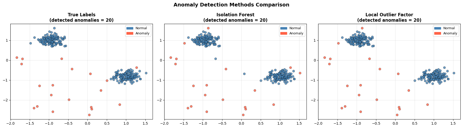
Isolation Forest      Anomaly F1 = 0.85  |  Precision = 0.85
LOF                   Anomaly F1 = 0.90  |  Precision = 0.90
Both methods recover most of the injected anomalies. The remaining misclassified points are either anomalies that landed inside a dense cluster by chance, or normal points near the edges of their clusters that look isolated.
6.3.3.5. Choosing a Method#
Situation |
Recommendation |
|---|---|
General tabular data |
Isolation Forest — fast, scalable, robust |
Anomalies relative to local neighbourhood |
LOF |
Univariate feature, Gaussian distribution |
Z-Score |
Explicit covariance structure known |
Elliptic Envelope |
Tip
The contamination parameter controls the fraction of data the model labels as anomalies. Setting it too low means anomalies go undetected; too high means many normal points get flagged. Calibrate it using domain knowledge about the expected anomaly rate.