6.2.2.7. Random Forest

Random Forest is the Bagging algorithm applied to classification trees - with one crucial twist: feature randomisation. Instead of just training each tree on a bootstrap sample, at every split the algorithm considers only a random subset of \(m\) features. This decorrelates the trees, making their errors more independent, so the majority vote is far more reliable than any individual tree.

The result is exactly the classification counterpart of Random Forest:

• Reduced variance from averaging many diverse trees

• Near-zero overfitting compared to a single deep tree

• Free out-of-bag (OOB) validation - each tree is tested on the ~37% of data it did not see during training

Random Forest is widely regarded as the best default classifier for tabular data.

---

The Math

Training:

1. For \(b = 1, \ldots, B\):

   1. Draw a bootstrap sample \(\mathcal{D}_b\) (same size as the training set, with replacement).

   2. Grow a full decision tree on \(\mathcal{D}_b\). At every split, sample \(m \leq p\) features and choose the best split only among those \(m\) features.

2. Store all \(B\) trees.

Prediction (majority vote):

\[\hat{y}_{\text{RF}}(\mathbf{x}) = \underset{c}{\arg\max}\;\sum_{b=1}^{B}\mathbf{1}\!\left[\hat{f}_b(\mathbf{x}) = c\right]\]

The default choice \(m = \lfloor\sqrt{p}\rfloor\) balances bias and variance in practice.

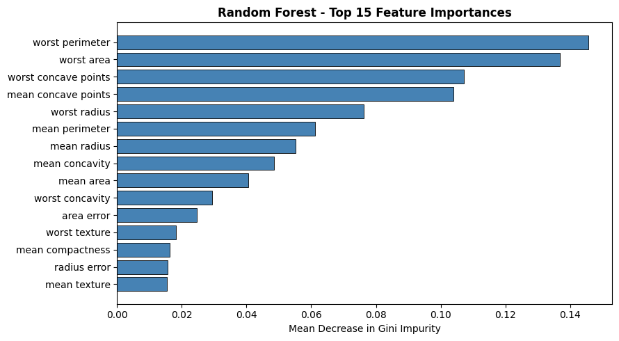
Feature importance is the mean decrease in Gini impurity across all splits on that feature, averaged over all trees.

Key hyperparameters:

Hyperparameter	Guidance
n_estimators	More trees → better, diminishing returns after ~200-500
max_features	'sqrt' (default) is robust; 1.0 = use all features = Bagging
max_depth	Default None (full depth); restrict if RAM is a concern
min_samples_leaf	Smooths individual trees; useful for noisy data
oob_score=True	Free out-of-bag validation estimate

---

In scikit-learn

from sklearn.ensemble import RandomForestClassifier

rf = RandomForestClassifier(
    n_estimators=200,
    max_features='sqrt',
    oob_score=True,
    random_state=42,
    n_jobs=-1
)
rf.fit(X_train, y_train)

No feature scaling is required - Random Forest inherits this property from decision trees.

---

Example

Show code cell source

Hide code cell source

import numpy as np
import pandas as pd
import matplotlib.pyplot as plt
from myst_nb import glue
from sklearn.ensemble import RandomForestClassifier
from sklearn.datasets import load_breast_cancer
from sklearn.model_selection import train_test_split
from sklearn.metrics import accuracy_score, roc_auc_score

np.random.seed(42)

# Shared dataset used throughout all Classification Algorithm pages
data = load_breast_cancer()
X, y = data.data, data.target   # 0 = malignant, 1 = benign
X_train, X_test, y_train, y_test = train_test_split(
    X, y, test_size=0.25, random_state=42, stratify=y)

from sklearn.ensemble import RandomForestClassifier

rf = RandomForestClassifier(n_estimators=200, max_features='sqrt',
                             oob_score=True, random_state=42, n_jobs=-1)
rf.fit(X_train, y_train)

train_acc = accuracy_score(y_train, rf.predict(X_train))
test_acc  = accuracy_score(y_test,  rf.predict(X_test))
test_auc  = roc_auc_score(y_test,   rf.predict_proba(X_test)[:, 1])

Random Forest achieves a test accuracy of 0.958 and AUC-ROC of 0.995. The OOB accuracy of 0.962 closely tracks the held-out test score - a useful sanity check that doesn’t require a separate validation split. Train accuracy of 1.0 is near perfect (full-depth trees memorise their bootstrap samples) but that does not imply the ensemble overfits.

Feature Importance

imp_df = pd.DataFrame({
    "Feature":    data.feature_names,
    "Importance": rf.feature_importances_,
}).sort_values("Importance", ascending=True).tail(15)

fig, ax = plt.subplots(figsize=(9, 5))
ax.barh(imp_df["Feature"], imp_df["Importance"],
        color='steelblue', edgecolor='black', linewidth=0.6)
ax.set_xlabel("Mean Decrease in Gini Impurity")
ax.set_title("Random Forest - Top 15 Feature Importances", fontweight='bold')
plt.tight_layout()
plt.show()

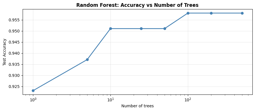
Number of Trees vs Accuracy

More trees always helps (or at worst, is neutral). Performance plateaus around 100–300 trees on most datasets.

n_values  = [1, 5, 10, 25, 50, 100, 200, 500]
test_accs = []

for n in n_values:
    m = RandomForestClassifier(n_estimators=n, max_features='sqrt',
                                random_state=42, n_jobs=-1)
    m.fit(X_train, y_train)
    test_accs.append(accuracy_score(y_test, m.predict(X_test)))

fig, ax = plt.subplots(figsize=(9, 4))
ax.semilogx(n_values, test_accs, 'o-', color='steelblue', lw=2)
ax.set_xlabel("Number of trees")
ax.set_ylabel("Test Accuracy")
ax.set_title("Random Forest: Accuracy vs Number of Trees", fontweight='bold')
ax.grid(True, alpha=0.3)
plt.tight_layout()
plt.show()