6.2.2.3. k-Nearest Neighbours Classification#
k-Nearest Neighbours (k-NN) is a lazy learner - there is no explicit training step. The algorithm simply stores the entire training set and, at prediction time, finds the \(k\) closest training examples to the query point. The predicted class is determined by a majority vote among those \(k\) neighbours.
This instance-based approach contrasts sharply with parametric models like Logistic Regression, which compress all learning into a fixed set of weights. k-NN retains the full training dataset and can represent arbitrarily complex decision boundaries - but that expressiveness comes with practical costs.
k-NN is an excellent sanity check and works well when the training set is large, the feature space is low-dimensional, and meaningful distances can be defined over the features.
The Math#
Prediction for a new point \(\mathbf{x}\):
Compute the distance from \(\mathbf{x}\) to every training point. The Euclidean distance is the default:
Let \(\mathcal{N}_k(\mathbf{x})\) be the set of indices of the \(k\) nearest training points.
Predict the majority class:
Key hyperparameters:
Hyperparameter |
Role |
|---|---|
|
Number of neighbours - larger \(k\) → smoother, less complex boundary |
|
Distance function: |
|
|
Scale sensitivity: Because k-NN uses raw distances, features with larger magnitudes dominate. Always scale features before applying k-NN.
Computational cost: Prediction is \(O(n \cdot p)\) per query (brute force). For large datasets use algorithm='ball_tree' or 'kd_tree'.
In scikit-learn#
from sklearn.neighbors import KNeighborsClassifier
from sklearn.preprocessing import StandardScaler
from sklearn.pipeline import Pipeline

model = Pipeline([
    ('scaler', StandardScaler()),
    ('knn',    KNeighborsClassifier(n_neighbors=5, weights='uniform'))
])
model.fit(X_train, y_train)
y_pred = model.predict(X_test)
Example#
from sklearn.neighbors import KNeighborsClassifier

knn = KNeighborsClassifier(n_neighbors=7, weights='uniform')
knn.fit(X_train_sc, y_train)

train_acc = accuracy_score(y_train, knn.predict(X_train_sc))
test_acc  = accuracy_score(y_test,  knn.predict(X_test_sc))
test_auc  = roc_auc_score(y_test,   knn.predict_proba(X_test_sc)[:, 1])
With \(k=7\), k-NN achieves a test accuracy of 0.979 and AUC-ROC of 0.992. The train accuracy of 0.974 is somewhat higher - a typical pattern because k-NN memorises the training set and can overfit with small \(k\).
Choosing k: The Bias–Variance Trade-off#
A small \(k\) (e.g. \(k=1\)) produces a very jagged, high-variance boundary. A large \(k\) smooths the boundary but introduces bias. Cross-validation over \(k\) is the standard way to find the sweet spot.
k_values    = list(range(1, 31))
train_accs  = []
test_accs   = []

for k in k_values:
    m = KNeighborsClassifier(n_neighbors=k)
    m.fit(X_train_sc, y_train)
    train_accs.append(accuracy_score(y_train, m.predict(X_train_sc)))
    test_accs.append(accuracy_score(y_test,   m.predict(X_test_sc)))

fig, ax = plt.subplots(figsize=(9, 4))
ax.plot(k_values, train_accs, 'o-', label='Train Accuracy', color='steelblue')
ax.plot(k_values, test_accs,  's-', label='Test Accuracy',  color='tomato')
ax.set_xlabel("Number of neighbours (k)")
ax.set_ylabel("Accuracy")
ax.set_title("k-NN: Accuracy vs k (Breast Cancer)", fontweight='bold')
ax.legend()
ax.grid(True, alpha=0.3)
plt.tight_layout()
plt.show()
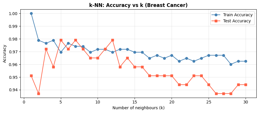
As \(k\) increases, train accuracy falls (less memorisation) while test accuracy first rises then plateaus or falls. The optimal \(k\) balances this trade-off.