DBSCAN: Density-Based Clustering

6.3.1.3. DBSCAN: Density-Based Clustering#

K-Means Clustering and Hierarchical Clustering clustering both assume that clusters are roughly convex and similarly sized. Real data rarely cooperates. Clusters can be crescent-shaped, ring-shaped, or embedded in a sea of noise.

DBSCAN (Density-Based Spatial Clustering of Applications with Noise) escapes these limitations entirely. It defines a cluster as a dense region of points separated from other dense regions by sparse space — no assumption about shape, and no requirement to specify \(k\) in advance.

As a bonus, DBSCAN naturally labels low-density points as noise, making it a useful detector of outliers at the same time.

The Intuition#

Think of a large party scattered across a park. Some people cluster tightly in conversation circles (dense regions); others wander alone between groups (sparse space). DBSCAN would identify the circles as clusters and the isolated wanderers as noise.

The algorithm classifies every point into one of three roles:

Core point — has at least min_samples neighbours within radius \(\varepsilon\).
Border point — within radius \(\varepsilon\) of a core point, but does not itself have enough neighbours to be core.
Noise point — neither core nor reachable from any core point.

Clusters are then built by connecting all core points that are within \(\varepsilon\) of each other, and attaching border points to their nearest cluster.

The Math#

\(\varepsilon\)-neighbourhood of point \(\mathbf{x}\):

\[N_\varepsilon(\mathbf{x}) = \{ \mathbf{x}' : d(\mathbf{x}, \mathbf{x}') \leq \varepsilon \}\]

A point \(\mathbf{x}\) is a core point if \(|N_\varepsilon(\mathbf{x})| \geq \text{min_samples}\).

Two core points \(\mathbf{p}\) and \(\mathbf{q}\) are in the same cluster if they are density-connected: there exists a chain of core points \(\mathbf{p} = \mathbf{z}_0, \mathbf{z}_1, \ldots, \mathbf{z}_m = \mathbf{q}\) where each consecutive pair satisfies \(d(\mathbf{z}_i, \mathbf{z}_{i+1}) \leq \varepsilon\).

Choosing \(\varepsilon\) — the k-nearest-neighbour distance plot:

For each point compute the distance to its \(k\)-th nearest neighbour (use \(k = \text{min_samples}\)).
Sort these distances in ascending order and plot them.
The \(\varepsilon\) value sits at the “elbow” of the curve — the point where distance starts rising sharply.

In scikit-learn#

from sklearn.cluster import DBSCAN
from sklearn.preprocessing import StandardScaler

scaler = StandardScaler()
X_sc   = scaler.fit_transform(X)

db     = DBSCAN(eps=0.5, min_samples=5)
labels = db.fit_predict(X_sc)
# labels == -1  →  noise points

Key parameters:

Parameter	Meaning
`eps`	Neighbourhood radius \(\varepsilon\)
`min_samples`	Minimum neighbours to be a core point; larger → stricter density requirement
`metric`	Distance metric (default `'euclidean'`)

Tip

Always standardise features first — DBSCAN is sensitive to the scale of the distance metric.
Noise points receive label -1. Check (labels == -1).sum() to see how many points were flagged as outliers.

Example#

Where DBSCAN Beats K-Means#

datasets = {
    'Crescent Moons': make_moons(n_samples=300, noise=0.07, random_state=42),
    'Concentric Rings': make_circles(n_samples=300, factor=0.5, noise=0.06, random_state=42),
}
settings = {
    'Crescent Moons':   dict(eps=0.25, min_samples=5),
    'Concentric Rings': dict(eps=0.18, min_samples=5),
}

fig, axes = plt.subplots(2, 3, figsize=(16, 9))

for row, (name, (X_raw, y_true)) in enumerate(datasets.items()):
    X_sc = StandardScaler().fit_transform(X_raw)

    # True labels
    axes[row, 0].scatter(X_sc[:, 0], X_sc[:, 1], c=y_true,
                         cmap='tab10', alpha=0.7, edgecolors='k', linewidths=0.3, s=45)
    axes[row, 0].set_title(f'{name}\nTrue Labels', fontweight='bold')

    # K-Means
    km_labels = KMeans(n_clusters=2, random_state=42, n_init=10).fit_predict(X_sc)
    axes[row, 1].scatter(X_sc[:, 0], X_sc[:, 1], c=km_labels,
                         cmap='tab10', alpha=0.7, edgecolors='k', linewidths=0.3, s=45)
    axes[row, 1].set_title(f'{name}\nK-Means (k=2)', fontweight='bold')

    # DBSCAN
    db_labels = DBSCAN(**settings[name]).fit_predict(X_sc)
    colors = np.where(db_labels == -1, 0.5, db_labels.astype(float))
    sc = axes[row, 2].scatter(X_sc[:, 0], X_sc[:, 1], c=db_labels,
                              cmap='tab10', alpha=0.7, edgecolors='k', linewidths=0.3, s=45)
    noise_n = (db_labels == -1).sum()
    axes[row, 2].set_title(f'{name}\nDBSCAN (noise={noise_n})', fontweight='bold')

for ax in axes.flatten():
    ax.grid(True, alpha=0.2)
    ax.set_xticks([]); ax.set_yticks([])

plt.suptitle('K-Means vs DBSCAN on Non-Convex Datasets', fontsize=14, fontweight='bold')
plt.tight_layout()
plt.show()

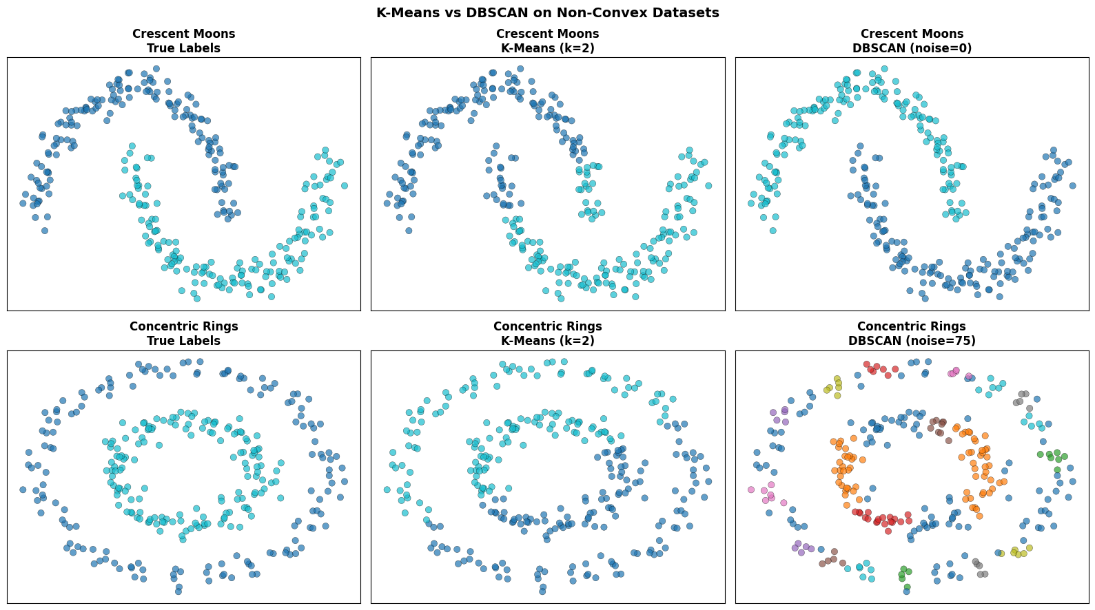
../../../../_images/f7a39f299f70f1317e47346035d340aeaffa09c332db847972de8211cc45470c.png

K-Means carves the space into two Voronoi regions and fails badly on both shapes. DBSCAN follows the density structure and recovers the correct partition.

Choosing eps with the k-NN Distance Plot#

from sklearn.neighbors import NearestNeighbors
from sklearn.datasets import make_moons

X_raw, _ = make_moons(n_samples=300, noise=0.07, random_state=42)
X_sc     = StandardScaler().fit_transform(X_raw)

# k = min_samples = 5
nbrs   = NearestNeighbors(n_neighbors=5).fit(X_sc)
dists, _ = nbrs.kneighbors(X_sc)
knn_dists = np.sort(dists[:, -1])   # distance to 5th nearest neighbour

fig, ax = plt.subplots(figsize=(9, 4))
ax.plot(knn_dists, linewidth=2, color='steelblue')
ax.axhline(y=0.25, color='tomato', linestyle='--', linewidth=1.5, label='eps = 0.25 (elbow)')
ax.set_xlabel('Points (sorted)', fontsize=12)
ax.set_ylabel('Distance to 5th neighbour', fontsize=12)
ax.set_title('k-NN Distance Plot — finding eps', fontsize=13, fontweight='bold')
ax.legend(); ax.grid(True, alpha=0.3)
plt.tight_layout()
plt.show()

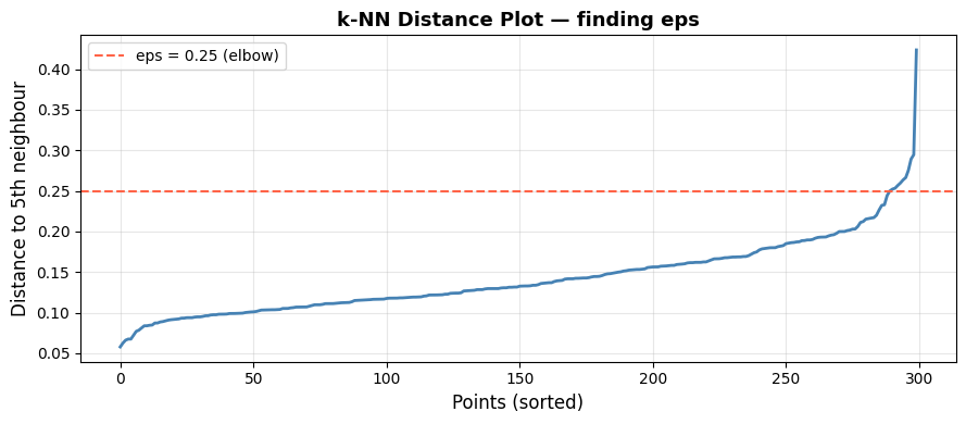
../../../../_images/00e95f042e71228d028bf062e56bf1715b5add774d623bf23c5c93084c021371.png

The elbow at approximately 0.25 is where the distance begins rising steeply. Setting eps just above this value includes genuine cluster members while excluding sparse noise points.

Strengths and Weaknesses#


Strengths	Finds arbitrarily shaped clusters; automatically identifies noise/outliers; no need to pre-specify \(k\); robust to outliers within clusters
Weaknesses	Sensitive to `eps` and `min_samples`; struggles with clusters of varying density; slow on very large datasets unless an index (ball tree, kd-tree) is used