5.3.4. Visualizing Relationships and Structure#
As the number of features in a dataset grows, understanding relationships through tables and statistics alone becomes increasingly difficult. Visualization provides an intuitive way to explore structure, patterns, and anomalies in data by projecting complex relationships into interpretable forms.
This section introduces common visualization techniques for exploratory analysis and shows how dimensionality reduction enables visualization of high-dimensional data.
5.3.4.1. Univariate and Bivariate Plots#
Visualization often begins with simple plots that reveal basic structure.
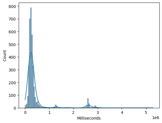
Histograms and Density Plots#
Histograms and kernel density estimates (KDEs) help visualize the distribution of individual numeric features. They are useful for identifying skewness, multimodality, and outliers.
import sqlite3
import pandas as pd
import matplotlib.pyplot as plt
import seaborn as sns

# Connect to Chinook sample database
conn = sqlite3.connect("../data/chinook.db")

# Load the 'tracks' table into a DataFrame
df_tracks = pd.read_sql_query("SELECT * FROM tracks", conn)
sns.histplot(df_tracks["Milliseconds"], kde=True)
<Axes: xlabel='Milliseconds', ylabel='Count'>
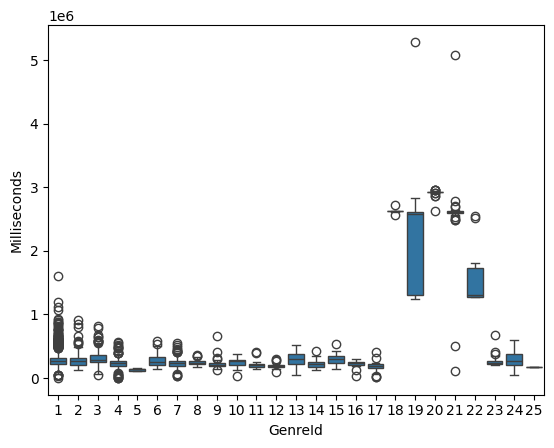
Box Plots#
Box plots summarize distribution using quartiles and highlight potential outliers. They are especially useful for comparing numeric features across categories.
sns.boxplot(x="GenreId", y="Milliseconds", data=df_tracks)
<Axes: xlabel='GenreId', ylabel='Milliseconds'>
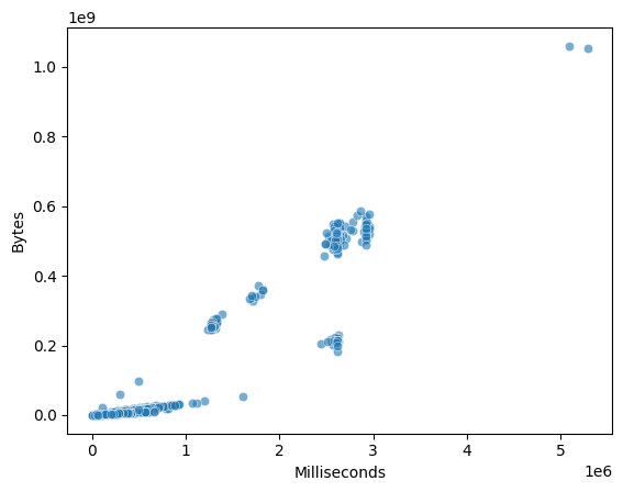
Scatter Plots#
Scatter plots visualize the relationship between two numeric features. They help identify trends, clusters, and nonlinear relationships.
sns.scatterplot(
    x="Milliseconds",
    y="Bytes",
    data=df_tracks,
    alpha=0.6
)
<Axes: xlabel='Milliseconds', ylabel='Bytes'>
5.3.4.2. Pairwise Relationship Plots#
When exploring relationships across multiple features, pairwise plots provide a compact overview.
Pair Plot#
A pair plot displays scatter plots for every pair of selected features along with univariate distributions on the diagonal.
selected_cols = ["Milliseconds", "Bytes", "UnitPrice"]
sns.pairplot(df_tracks[selected_cols], diag_kind="kde")
<seaborn.axisgrid.PairGrid at 0x7fd2d8a22900>
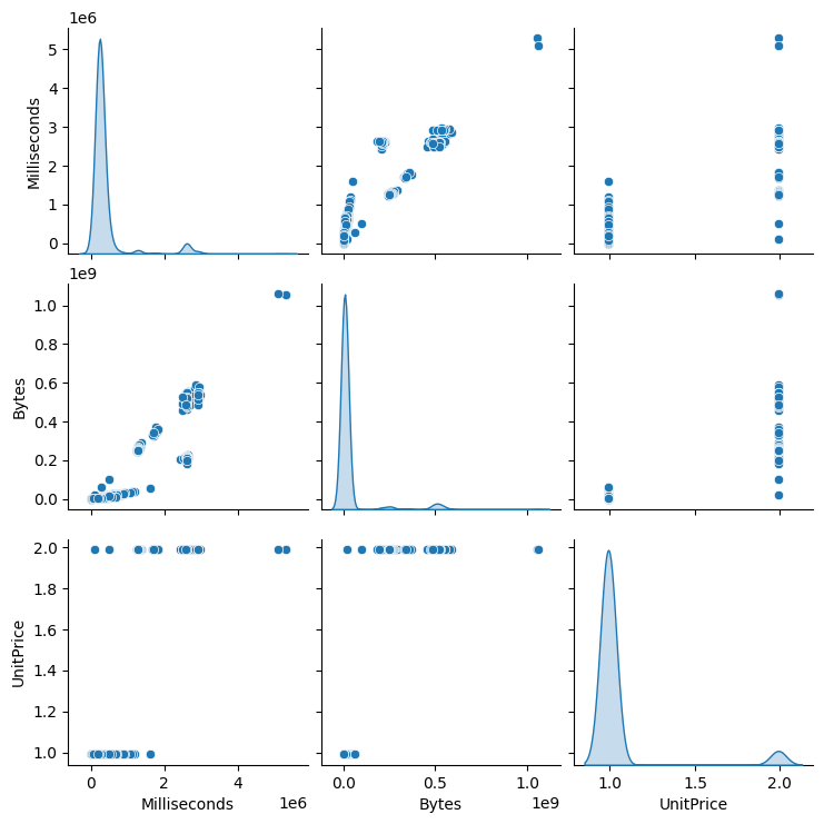
Pair plots are most effective for small to medium-sized datasets with a limited number of numeric features.
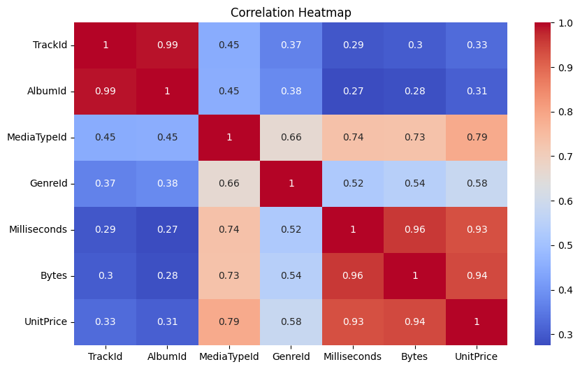
5.3.4.3. Correlation Heatmaps#
Correlation heatmaps provide a visual summary of linear relationships between many features at once.
import matplotlib.pyplot as plt

corr = df_tracks.corr(numeric_only=True)

plt.figure(figsize=(10, 6))
sns.heatmap(corr, annot=True, cmap="coolwarm")
plt.title("Correlation Heatmap")
plt.show()
Visualizing these correlations makes comparison easier:
target = "UnitPrice"
correlations = corr[target].drop(target)
correlations.sort_values().plot(kind="barh", figsize=(8, 6))
plt.xlabel("Correlation")
plt.title(f"Feature Correlation with '{target}'")
plt.show()
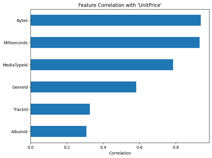
Features with very weak correlation to the target may contribute little to linear models, while highly correlated features may require further inspection for redundancy.
These plots help identify redundant features and strong dependencies.
5.3.4.4. Visualizing High-Dimensional Data#
As dimensionality increases, direct visualization becomes impractical. Dimensionality reduction techniques project high-dimensional data into lower dimensions while preserving important structure.
5.3.4.5. PCA for Visualization#
Principal Component Analysis (PCA) is a linear dimensionality reduction technique that projects data onto directions of maximum variance.
Key properties:
Captures global structure
Components are orthogonal
Sensitive to scale
Note
Features should be standardized before applying PCA to prevent scale dominance.
from sklearn.preprocessing import StandardScaler
from sklearn.decomposition import PCA

features = df_tracks.select_dtypes(include="number").drop(columns=["UnitPrice"], errors="ignore")
X_scaled = StandardScaler().fit_transform(features)

pca = PCA(n_components=2)
X_pca = pca.fit_transform(X_scaled)
sns.scatterplot(x=X_pca[:, 0], y=X_pca[:, 1])
plt.xlabel("Principal Component 1")
plt.ylabel("Principal Component 2")
plt.title("PCA Projection")
plt.show()
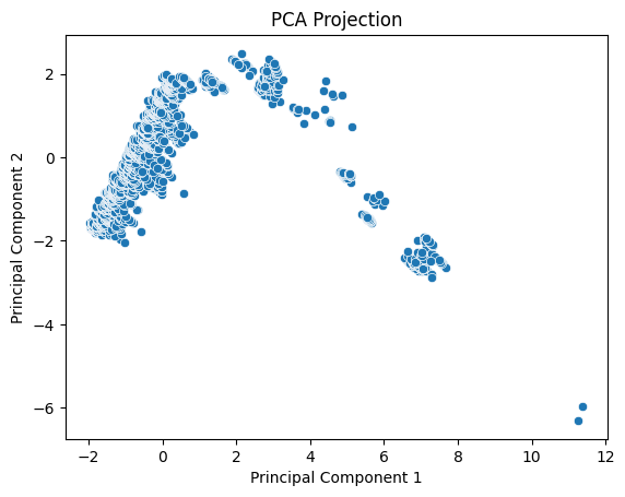
PCA allows us to visualize dominant variation and detect structure such as clusters or gradients.
5.3.4.6. Summary#
Visualization is a central component of exploratory data analysis. Simple plots reveal distributions and pairwise relationships, while dimensionality reduction techniques such as PCA make it possible to explore structure in high-dimensional data.
Together, these tools complement statistical measures by providing intuitive insight into patterns, relationships, and anomalies that may not be obvious from numbers alone.