6.2.1.4. Support Vector Regression

Support Vector Regression (SVR) extends the Support Vector Machine idea from classification to continuous outputs. The key intuition is different from ordinary least squares: instead of minimising the total squared error for every point, SVR tries to fit the data within a tube of width \(\varepsilon\) around the prediction.

• Points inside the tube incur zero loss - small errors are tolerated.

• Points outside the tube are penalised linearly with distance from the tube boundary.

This tolerance zone makes SVR naturally robust to small amounts of noise. The points that actually sit on or outside the tube boundary are the support vectors - they alone determine the model. All other points are irrelevant to the solution.

The second powerful feature of SVR is the kernel trick: by applying a non-linear transformation to the input space, SVR can fit curved, complex relationships without explicitly engineering polynomial or interaction features.

---

The Math

SVR solves the following optimisation problem:

\[\min_{\boldsymbol{w}, b,\,\xi,\xi^*} \frac{1}{2}\|\boldsymbol{w}\|^2 + C \sum_{i=1}^{n}(\xi_i + \xi_i^*)\]

subject to:

\[y_i - \langle \boldsymbol{w}, \boldsymbol{x}_i \rangle - b \;\leq\; \varepsilon + \xi_i, \quad \langle \boldsymbol{w}, \boldsymbol{x}_i \rangle + b - y_i \;\leq\; \varepsilon + \xi_i^*\]

where \(\xi_i, \xi_i^* \geq 0\) are slack variables that allow points to sit outside the tube.

The RBF (Radial Basis Function) kernel maps inputs into an infinite-dimensional space, enabling non-linear fits:

\[K(\mathbf{x}, \mathbf{x}') = \exp\!\left(-\gamma \|\mathbf{x} - \mathbf{x}'\|^2\right)\]

Key hyperparameters:

Hyperparameter	Role
C	Regularization - high C fits training data tightly; low C is smoother
epsilon (\(\varepsilon\))	Tube half-width - errors within this band are ignored entirely
kernel	Feature transformation: linear, rbf, poly
gamma	RBF width - high gamma → narrow Gaussians, complex boundary

---

In scikit-learn

SVR requires feature scaling - the optimisation is sensitive to feature magnitudes. Always wrap it in a Pipeline with StandardScaler.

from sklearn.svm import SVR
from sklearn.pipeline import Pipeline
from sklearn.preprocessing import StandardScaler

svr = Pipeline([
    ('scaler', StandardScaler()),
    ('svr',    SVR(kernel='rbf', C=100, epsilon=5))
])
svr.fit(X_train, y_train)

---

Example

Show code cell source

Hide code cell source

import numpy as np
import pandas as pd
import matplotlib.pyplot as plt
from myst_nb import glue
from sklearn.svm import SVR
from sklearn.pipeline import Pipeline
from sklearn.preprocessing import StandardScaler
from sklearn.model_selection import train_test_split
from sklearn.metrics import mean_squared_error, r2_score
from sklearn.datasets import make_regression

np.random.seed(42)

X, y = make_regression(n_samples=300, n_features=10, n_informative=6,
                        noise=25, random_state=42)
X_train, X_test, y_train, y_test = train_test_split(
    X, y, test_size=0.25, random_state=42)

svr = Pipeline([
    ('scaler', StandardScaler()),
    ('svr',    SVR(kernel='rbf', C=100, epsilon=5))
])
svr.fit(X_train, y_train)

train_r2  = r2_score(y_train, svr.predict(X_train))
test_r2   = r2_score(y_test,  svr.predict(X_test))
test_rmse = np.sqrt(mean_squared_error(y_test, svr.predict(X_test)))

print(f"Train R²  : {train_r2:.3f}")
print(f"Test  R²  : {test_r2:.3f}")
print(f"Test  RMSE: {test_rmse:.1f}")

Train R²  : 0.945
Test  R²  : 0.853
Test  RMSE: 68.1

SVR achieves a test \(R^2\) of 0.853 and RMSE of 68.1. The train \(R^2\) is 0.945.

The \(\varepsilon\)-Tube on 1-D Data

To understand how the tube and support vectors work, it is easiest to visualise SVR on a one-dimensional sine curve:

np.random.seed(1)
X_1d = np.sort(np.random.uniform(0, 6, 60)).reshape(-1, 1)
y_1d = 2 * np.sin(X_1d.ravel()) + np.random.normal(0, 0.4, 60)

svr_demo = SVR(kernel='rbf', C=10, epsilon=0.3)
svr_demo.fit(X_1d, y_1d)

Xp = np.linspace(0, 6, 300).reshape(-1, 1)
yp = svr_demo.predict(Xp)

plt.figure(figsize=(10, 5))
plt.scatter(X_1d, y_1d, zorder=3, edgecolors='k', linewidths=0.5,
            alpha=0.7, label='Training data', color='steelblue')
plt.plot(Xp, yp, 'r-', linewidth=2.5, label='SVR prediction', zorder=4)
plt.fill_between(Xp.ravel(), yp - 0.3, yp + 0.3,
                 alpha=0.2, color='red', label='ε-tube (ε=0.3)')

sv_mask = np.zeros(len(X_1d), dtype=bool)
sv_mask[svr_demo.support_] = True
plt.scatter(X_1d[sv_mask], y_1d[sv_mask], s=120, facecolors='none',
            edgecolors='blue', linewidths=2, zorder=5,
            label=f'Support vectors ({sv_mask.sum()})')

plt.xlabel('X', fontsize=12)
plt.ylabel('y', fontsize=12)
plt.title('SVR - ε-Tube and Support Vectors', fontsize=13, fontweight='bold')
plt.legend(fontsize=10)
plt.grid(True, alpha=0.3)
plt.tight_layout()
plt.show()

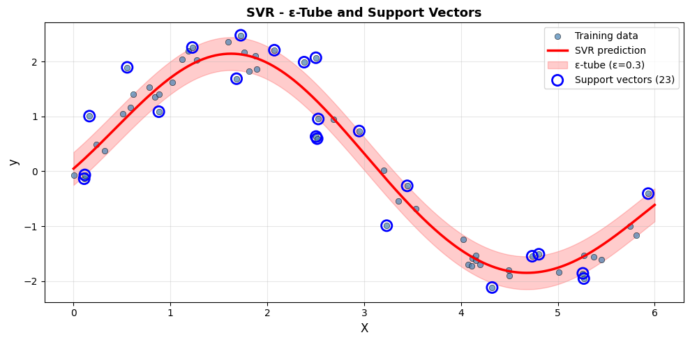
Only 23 of the 60 training points (38.3%) become support vectors. The rest lie inside the tube and have no effect on the model - this is the “support” in SVR.

Hyperparameter Sensitivity - C and Epsilon

Show code cell source

Hide code cell source

fig, axes = plt.subplots(2, 3, figsize=(15, 8), sharey=True)

C_vals = [0.1, 10, 500]
eps_vals = [0.1, 1.0, 3.0]

# Vary C (top row)
for ax, C_val in zip(axes[0], C_vals):
    m = SVR(kernel='rbf', C=C_val, epsilon=0.3)
    m.fit(X_1d, y_1d)
    yp_ = m.predict(Xp)
    ax.scatter(X_1d, y_1d, s=15, alpha=0.5, color='steelblue')
    ax.plot(Xp, yp_, 'r-', linewidth=2)
    ax.fill_between(Xp.ravel(), yp_ - 0.3, yp_ + 0.3, alpha=0.15, color='red')
    ax.set_title(f'C={C_val}  (ε=0.3)', fontsize=10, fontweight='bold')
    ax.grid(True, alpha=0.3)

# Vary epsilon (bottom row)
for ax, eps_val in zip(axes[1], eps_vals):
    m = SVR(kernel='rbf', C=10, epsilon=eps_val)
    m.fit(X_1d, y_1d)
    yp_ = m.predict(Xp)
    ax.scatter(X_1d, y_1d, s=15, alpha=0.5, color='steelblue')
    ax.plot(Xp, yp_, 'r-', linewidth=2)
    ax.fill_between(Xp.ravel(), yp_ - eps_val, yp_ + eps_val,
                    alpha=0.15, color='red')
    ax.set_title(f'ε={eps_val}  (C=10)', fontsize=10, fontweight='bold')
    ax.grid(True, alpha=0.3)

axes[0][0].set_ylabel('y', fontsize=11)
axes[1][0].set_ylabel('y', fontsize=11)
fig.suptitle('SVR Hyperparameter Sensitivity',
             fontsize=13, fontweight='bold', y=1.01)
plt.tight_layout()
plt.show()

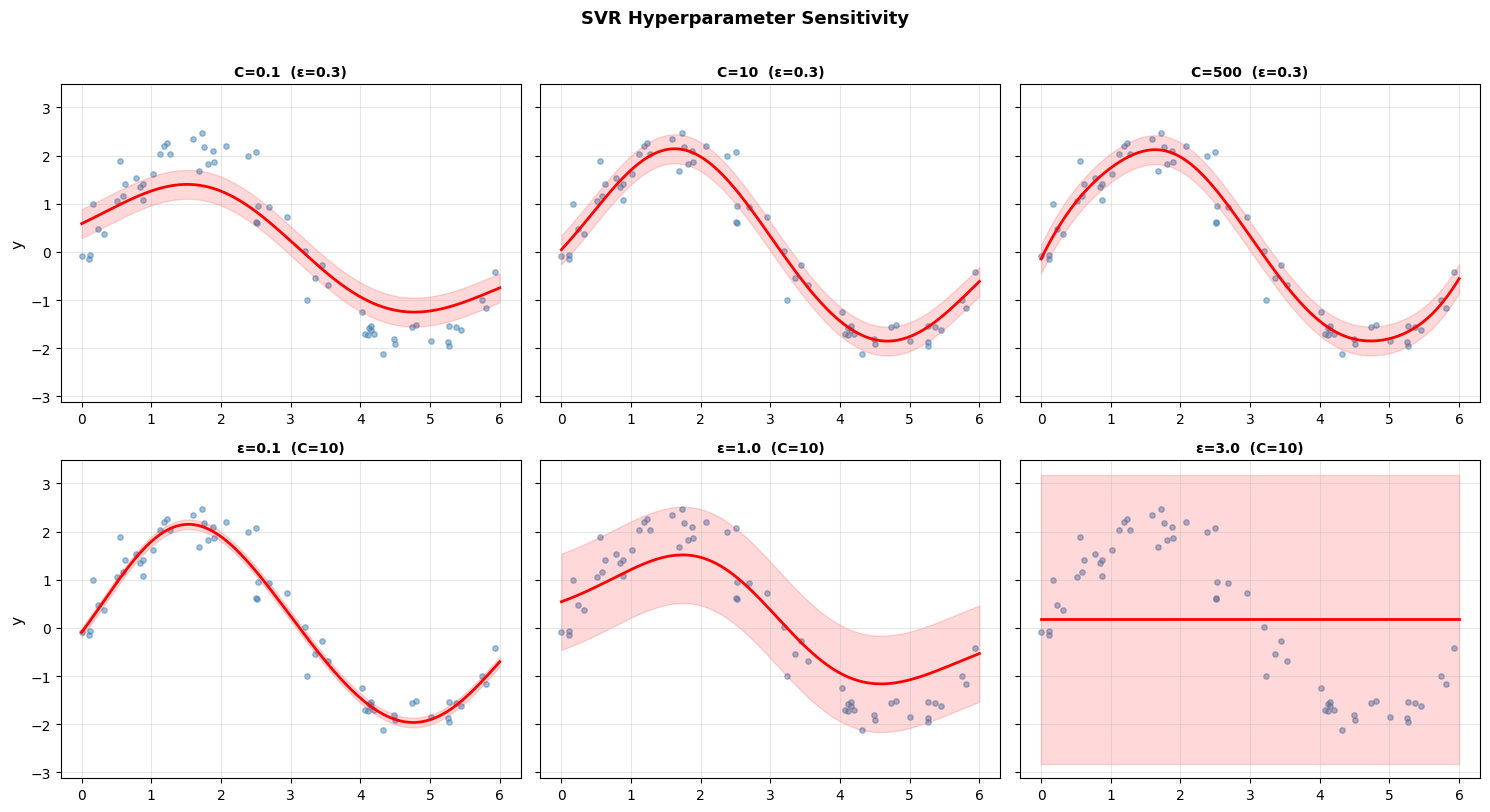
Top row (varying C): Low C produces a smooth, underfit curve. High C fits the training data very tightly, risking overfitting.

Bottom row (varying ε): Small ε uses many support vectors (narrow tolerance). Large ε uses fewer and produces a smoother, coarser fit.

---

Strengths and Weaknesses

Strengths	Handles non-linear relationships via kernels; robust with the ε-tube; effective in high-dimensional spaces
Weaknesses	Slow on large datasets (\(O(n^2)\)–\(O(n^3)\)); requires feature scaling; less interpretable; hyperparameter tuning critical

Tip

SVR excels on small-to-medium datasets (< 10k samples) with non-linear relationships. For large datasets consider Gradient Boosting or Random Forest instead.