6.2.2.5. Decision Tree Classifier#
A decision tree classifier partitions the feature space into axis-aligned regions by asking a series of yes/no questions - a flowchart from root to leaf. At every internal node the tree asks: “Is feature \(j\) above threshold \(t\)?” A sample follows one branch, and the same question is repeated until a leaf is reached. The predicted class at that leaf is the majority class of all training samples in that region.
Unlike Logistic Regression, which creates a single linear boundary, a decision tree can carve out arbitrarily complex, non-linear regions. Like the decision-tree-regressor, the central tension is the bias–variance trade-off: deeper trees can perfectly memorise training data but generalise poorly; shallow trees are robust but may underfit.
The Math#
At each node, the algorithm searches all features \(j\) and thresholds \(t\) for the split that maximally reduces impurity. The two standard impurity measures are:
Gini impurity (default in scikit-learn):
Entropy (information gain):
where \(p_c\) is the proportion of class \(c\) samples in node \(S\). A node is pure (Gini = 0, \(H\) = 0) when all samples belong to one class.
The information gain of a split is:
The prediction at each leaf is the majority class; ties are broken arbitrarily.
Key hyperparameters:
Hyperparameter |
Effect |
|---|---|
|
Maximum levels of splits - primary complexity control |
|
Minimum training samples per leaf - higher → smoother |
|
|
|
Number of features considered per split |
In scikit-learn#
from sklearn.tree import DecisionTreeClassifier

tree = DecisionTreeClassifier(max_depth=5, min_samples_leaf=5,
                               criterion='gini', random_state=42)
tree.fit(X_train, y_train)
No feature scaling required - trees split on rank order, not magnitude.
Example#
from sklearn.tree import DecisionTreeClassifier

tree = DecisionTreeClassifier(max_depth=5, random_state=42)
tree.fit(X_train, y_train)

train_acc = accuracy_score(y_train, tree.predict(X_train))
test_acc  = accuracy_score(y_test,  tree.predict(X_test))
test_auc  = roc_auc_score(y_test,   tree.predict_proba(X_test)[:, 1])
With max_depth=5, the tree achieves a test accuracy of 0.937 and AUC-ROC of 0.919. The train accuracy of 0.995 is higher - a typical sign of overfitting in unconstrained trees.
Visualising the Tree Structure#
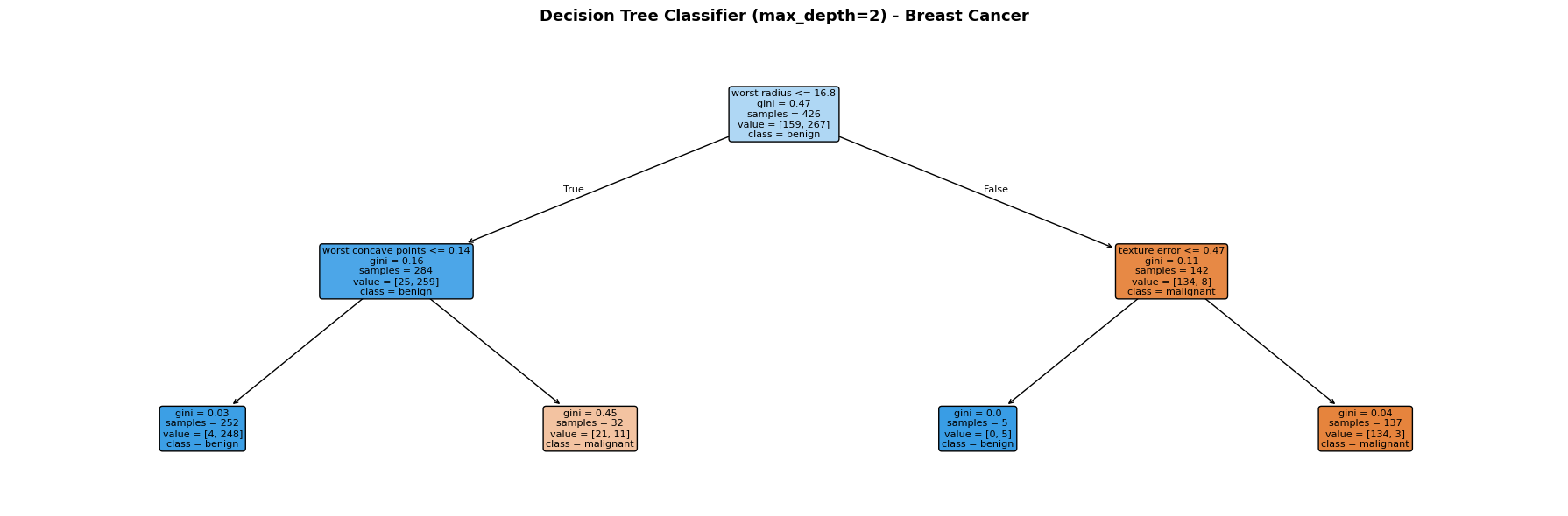
Each node shows the splitting rule, Gini impurity, number of samples, and class distribution. Leaf nodes are colour-coded by the predicted class (orange = malignant, blue = benign).
The Bias–Variance Trade-off Across Depths#
depths = [1, 2, 3, 5, 8, 12, None]

rows = []
for d in depths:
    m = DecisionTreeClassifier(max_depth=d, random_state=42)
    m.fit(X_train, y_train)
    rows.append({
        "max_depth": str(d),
        "Train Accuracy": round(accuracy_score(y_train, m.predict(X_train)), 3),
        "Test Accuracy":  round(accuracy_score(y_test,  m.predict(X_test)),  3),
        "Test AUC":       round(roc_auc_score(y_test,   m.predict_proba(X_test)[:, 1]), 3),
    })

pd.DataFrame(rows)
| max_depth | Train Accuracy | Test Accuracy | Test AUC | |
|---|---|---|---|---|
| 0 | 1 | 0.923 | 0.923 | 0.908 |
| 1 | 2 | 0.958 | 0.909 | 0.938 |
| 2 | 3 | 0.977 | 0.944 | 0.946 |
| 3 | 5 | 0.995 | 0.937 | 0.919 |
| 4 | 8 | 1.000 | 0.923 | 0.923 |
| 5 | 12 | 1.000 | 0.923 | 0.923 |
| 6 | None | 1.000 | 0.923 | 0.923 |
Shallow trees underfit; very deep trees memorise the training set. The sweet spot (here around max_depth=5) balances training fit against generalisation.