6.2.1.7. Random Forest

Random Forest is the definitive Bagging algorithm - and the go-to non-linear model for most tabular regression problems. It starts from the same idea as Bagging (see Ensemble Methods): grow many decision trees on bootstrap samples and average their predictions. But it adds one critical twist that makes it far more powerful: feature randomisation.

At each split inside every tree, the algorithm considers only a random subset of \(m\) features (not all \(p\) features). This decorrelates the trees. Without feature randomisation, if one feature is a very strong predictor, almost every tree would split on it first - the trees would look very similar and averaging them would provide little benefit. By forcing each tree to use a random feature subset, trees must find different paths through the data and end up making more independent errors.

The result is:

• Reduced variance from averaging many diverse trees

• Near-zero overfitting - unlike a single deep tree, the forest is robust

• Free validation via out-of-bag (OOB) samples - each tree is validated on the ~37% of data it did not see during training

---

The Math

Training algorithm:

1. For \(b = 1, \ldots, B\):

   1. Draw a bootstrap sample \(\mathcal{D}_b\) of size \(n\) from the training data.

   2. Grow a full (deep) decision tree on \(\mathcal{D}_b\). At every split, randomly sample \(m \leq p\) features and find the best split only among those \(m\) features.

2. Store all \(B\) trees.

Prediction:

\[\hat{y}_{\text{RF}}(\mathbf{x}) = \frac{1}{B}\sum_{b=1}^{B} \hat{f}_b(\mathbf{x})\]

The default choice of \(m = \sqrt{p}\) balances bias and variance well in practice.

Feature importance is computed as the mean decrease in impurity (MSE) across all splits on that feature, averaged over all trees.

Key hyperparameters:

Hyperparameter	Guidance
n_estimators	More is better up to a point; 100–500 is usually sufficient
max_features	"sqrt" (default) balances bias-variance; 1.0 = use all features
max_depth	Default None (full depth) works well; restrict if RAM is a concern
min_samples_leaf	Higher → smoother individual trees; useful for noisy targets
oob_score=True	Enables a free out-of-bag validation estimate

---

In scikit-learn

from sklearn.ensemble import RandomForestRegressor

rf = RandomForestRegressor(
    n_estimators=200,
    max_features='sqrt',
    oob_score=True,
    random_state=42,
    n_jobs=-1       # use all CPU cores
)
rf.fit(X_train, y_train)
print(f"OOB R²: {rf.oob_score_:.3f}")   # free estimate of test performance

No feature scaling is needed - Random Forest inherits this property from decision trees.

---

Example

Show code cell source

Hide code cell source

import numpy as np
import pandas as pd
import matplotlib.pyplot as plt
from myst_nb import glue
from sklearn.ensemble import RandomForestRegressor
from sklearn.model_selection import train_test_split
from sklearn.metrics import mean_squared_error, r2_score
from sklearn.datasets import make_regression

np.random.seed(42)

X, y = make_regression(n_samples=300, n_features=10, n_informative=6,
                        noise=25, random_state=42)
X_train, X_test, y_train, y_test = train_test_split(
    X, y, test_size=0.25, random_state=42)

rf = RandomForestRegressor(n_estimators=200, max_features='sqrt',
                           oob_score=True, random_state=42, n_jobs=-1)
rf.fit(X_train, y_train)

train_r2  = r2_score(y_train, rf.predict(X_train))
test_r2   = r2_score(y_test,  rf.predict(X_test))
test_rmse = np.sqrt(mean_squared_error(y_test, rf.predict(X_test)))
oob_r2    = rf.oob_score_

print(f"Train R²  : {train_r2:.3f}")
print(f"Test  R²  : {test_r2:.3f}")
print(f"OOB   R²  : {oob_r2:.3f}  ← free estimate, no test data used")
print(f"Test  RMSE: {test_rmse:.1f}")

Train R²  : 0.963
Test  R²  : 0.713
OOB   R²  : 0.732  ← free estimate, no test data used
Test  RMSE: 95.3

The forest achieves a test \(R^2\) of 0.713 and an OOB \(R^2\) of 0.732. Notice how closely OOB and test performance agree - the OOB estimate is a reliable free substitute for a separate validation set.

Feature Importance

Random Forest provides interpretable feature importance scores as a by-product of training - no extra computation required:

Show code cell source

Hide code cell source

imp = pd.Series(rf.feature_importances_,
                index=[f"Feature {i}" for i in range(X.shape[1])])
imp = imp.sort_values(ascending=False)

fig, ax = plt.subplots(figsize=(9, 4))
colors = ["#2ecc71" if i < 6 else "#e74c3c" for i in range(len(imp))]
imp.plot(kind="bar", ax=ax, edgecolor="black", alpha=0.85, color=colors)
ax.set_ylabel("Mean impurity decrease", fontsize=11)
ax.set_title("Random Forest - Feature Importances", fontsize=13, fontweight="bold")
ax.set_xticklabels(imp.index, rotation=45, ha="right")
ax.grid(True, alpha=0.3, axis="y")

from matplotlib.patches import Patch
legend_elements = [Patch(facecolor="#2ecc71", label="Informative (6)"),
                   Patch(facecolor="#e74c3c", label="Non-informative (4)")]
ax.legend(handles=legend_elements, fontsize=10)

plt.tight_layout()
plt.show()

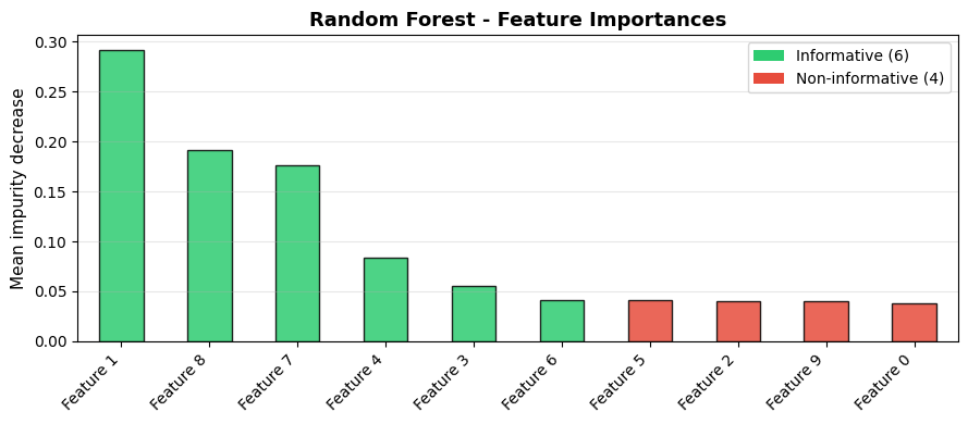
The most important feature is Feature 1 with an importance score of 0.292. The 4 non-informative features (shown in red) cluster at the bottom - Random Forest effectively deprioritises them.

Performance Stabilises with More Trees

Show code cell source

Hide code cell source

tree_counts = [1, 5, 10, 25, 50, 100, 200, 400]
train_scores, test_scores = [], []

for n in tree_counts:
    rf_n = RandomForestRegressor(n_estimators=n, random_state=42, n_jobs=-1)
    rf_n.fit(X_train, y_train)
    train_scores.append(rf_n.score(X_train, y_train))
    test_scores.append(rf_n.score(X_test, y_test))

fig, ax = plt.subplots(figsize=(10, 4))
ax.plot(tree_counts, train_scores, "o-", linewidth=2, label="Train R²")
ax.plot(tree_counts, test_scores,  "s--", linewidth=2, label="Test R²")
ax.set_xlabel("Number of Trees", fontsize=12)
ax.set_ylabel("R²", fontsize=12)
ax.set_title("Random Forest - Performance vs Number of Trees",
             fontsize=13, fontweight="bold")
ax.legend(fontsize=11)
ax.grid(True, alpha=0.3)
plt.tight_layout()
plt.show()

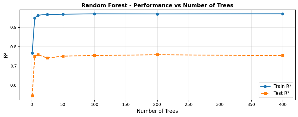
Test performance plateaus around 100–200 trees. Adding more trees beyond this point yields diminishing returns - the forest is already stable.

Effect of max_features on the Bias–Variance Balance

Show code cell source

Hide code cell source

mf_options = [1, 2, 3, 5, 7, 10]   # number of features considered at each split
mf_train, mf_test = [], []

for mf in mf_options:
    rf_mf = RandomForestRegressor(n_estimators=200, max_features=mf,
                                   random_state=42, n_jobs=-1)
    rf_mf.fit(X_train, y_train)
    mf_train.append(rf_mf.score(X_train, y_train))
    mf_test.append(rf_mf.score(X_test, y_test))

fig, ax = plt.subplots(figsize=(9, 4))
ax.plot(mf_options, mf_train, "o-", linewidth=2, label="Train R²")
ax.plot(mf_options, mf_test,  "s--", linewidth=2, label="Test R²")
ax.axvline(int(np.sqrt(X.shape[1])), color="red", linestyle=":",
           linewidth=1.5, label=f"√p ≈ {int(np.sqrt(X.shape[1]))}")
ax.set_xlabel("max_features  (features per split)", fontsize=12)
ax.set_ylabel("R²", fontsize=12)
ax.set_title("Random Forest - Effect of max_features",
             fontsize=13, fontweight="bold")
ax.legend(fontsize=11)
ax.grid(True, alpha=0.3)
plt.tight_layout()
plt.show()

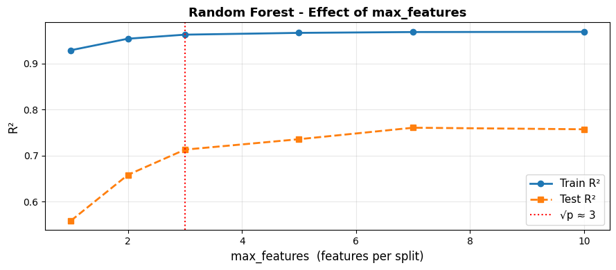
Using fewer features per split (left side) makes trees more diverse but individually weaker - higher bias, lower variance. Using all features (max_features=10) removes the decorrelation benefit. The default \(\sqrt{p}\) sits near the sweet spot.

---

Strengths and Weaknesses

Strengths	Excellent out-of-the-box performance; handles non-linearity; free OOB validation; robust to outliers and missing values; feature importance
Weaknesses	Less interpretable than a single tree; slower to train/predict than linear models; can overfit on very noisy data with too many trees

Tip

Random Forest is one of the best default models for tabular regression. Start here when a linear model under-performs and you need non-linear power with minimal tuning.