6.2.2.8. Boosting

All ensemble methods up to Random Forest train their models in parallel and aggregate the results. Boosting is fundamentally different: weak learners are trained sequentially, each one correcting the mistakes made by the previous ensemble.

The analogy is a student who reviews past exam papers: instead of studying broadly, they focus on the questions they got wrong last time. Sequential error correction means boosting reduces bias (the ensemble becomes increasingly accurate), whereas parallel aggregation primarily reduces variance.

Two algorithms dominate:

Algorithm	How the next learner is targeted
AdaBoost	Re-weights training samples - hard examples get higher weight
Gradient Boosting	Fits the next tree to the pseudo-residuals (negative gradient of the loss)

---

AdaBoost

The Math

AdaBoost trains a sequence of weak learners \(h_1, \ldots, h_M\) (typically decision stumps - trees of depth 1). After each round, misclassified samples receive higher weights so the next learner focuses on them.

1. Initialise equal sample weights \(w_i = 1/n\).

2. For \(m = 1, \ldots, M\):

   • a. Fit \(h_m\) on the weighted training set.

   • b. Compute weighted error: \(\varepsilon_m = \sum_i w_i \cdot \mathbf{1}[h_m(\mathbf{x}_i) \neq y_i]\).

   • c. Compute learner weight: \(\alpha_m = \frac{1}{2}\ln\!\frac{1-\varepsilon_m}{\varepsilon_m}\).

   • d. Update sample weights: increase for misclassified, decrease for correct.

3. Final prediction: \(\hat{y} = \mathrm{sign}\!\left(\sum_{m}\alpha_m h_m(\mathbf{x})\right)\).

Learners with lower error receive higher \(\alpha_m\) and dominate the final vote.

---

Gradient Boosting

The Math

Gradient Boosting frames boosting as gradient descent in function space. At each step, fit a tree to the negative gradient of the loss with respect to the current prediction.

For binary cross-entropy, the update is:

\[F_m(\mathbf{x}) = F_{m-1}(\mathbf{x}) + \eta \cdot h_m(\mathbf{x})\]

where \(h_m\) is fitted to the pseudo-residuals \(r_i = -\frac{\partial \mathcal{L}(y_i, F_{m-1}(\mathbf{x}_i))}{\partial F_{m-1}(\mathbf{x}_i)}\), and \(\eta\) is the learning rate (shrinkage).

Lower learning rates require more boosting rounds but generally generalise better - controlled by learning_rate and n_estimators.

---

In scikit-learn

from sklearn.ensemble import AdaBoostClassifier, GradientBoostingClassifier
from sklearn.tree import DecisionTreeClassifier

ada = AdaBoostClassifier(
    estimator=DecisionTreeClassifier(max_depth=1),   # stump
    n_estimators=100,
    learning_rate=1.0,
    random_state=42
)

gb = GradientBoostingClassifier(
    n_estimators=200,
    learning_rate=0.05,
    max_depth=3,
    random_state=42
)

Key hyperparameters:

Hyperparameter	Role
n_estimators	Number of boosting rounds
learning_rate	Shrinkage per round - lower → more rounds needed, often better generalisation
max_depth	Depth of each weak learner - shallow trees (1–5) are standard
estimator (AdaBoost)	The weak learner type

---

Example

Show code cell source

Hide code cell source

import numpy as np
import pandas as pd
import matplotlib.pyplot as plt
from myst_nb import glue
from sklearn.ensemble import AdaBoostClassifier, GradientBoostingClassifier
from sklearn.tree import DecisionTreeClassifier
from sklearn.datasets import load_breast_cancer
from sklearn.model_selection import train_test_split
from sklearn.metrics import accuracy_score, roc_auc_score

np.random.seed(42)

# Shared dataset used throughout all Classification Algorithm pages
data = load_breast_cancer()
X, y = data.data, data.target   # 0 = malignant, 1 = benign
X_train, X_test, y_train, y_test = train_test_split(
    X, y, test_size=0.25, random_state=42, stratify=y)

from sklearn.ensemble import AdaBoostClassifier, GradientBoostingClassifier
from sklearn.tree import DecisionTreeClassifier

ada = AdaBoostClassifier(
    estimator=DecisionTreeClassifier(max_depth=1),
    n_estimators=100, learning_rate=0.5, random_state=42)
ada.fit(X_train, y_train)

gb = GradientBoostingClassifier(
    n_estimators=200, learning_rate=0.05, max_depth=3, random_state=42)
gb.fit(X_train, y_train)

for name, model in [("AdaBoost", ada), ("GradientBoosting", gb)]:
    tr = accuracy_score(y_train, model.predict(X_train))
    te = accuracy_score(y_test,  model.predict(X_test))
    au = roc_auc_score(y_test,   model.predict_proba(X_test)[:, 1])
    print(f"{name:20s}  Train={tr:.3f}  Test={te:.3f}  AUC={au:.3f}")

AdaBoost              Train=1.000  Test=0.965  AUC=0.988
GradientBoosting      Train=1.000  Test=0.958  AUC=0.993

AdaBoost achieves a test accuracy of 0.965 (AUC 0.988). Gradient Boosting achieves 0.958 (AUC 0.993). Gradient Boosting typically matches or surpasses AdaBoost on most tabular datasets at the cost of more hyperparameters to tune.

Learning Curves: Staged Predictions

Both algorithms expose their staged predictions, allowing us to plot how test accuracy evolves with each additional boosting round.

# AdaBoost staged predictions
ada_stage_test = [accuracy_score(y_test, y_pred)
                  for y_pred in ada.staged_predict(X_test)]
ada_stage_train = [accuracy_score(y_train, y_pred)
                   for y_pred in ada.staged_predict(X_train)]

# GradientBoosting staged predictions
gb_stage_test  = [accuracy_score(y_test,  y_pred)
                  for y_pred in gb.staged_predict(X_test)]
gb_stage_train = [accuracy_score(y_train, y_pred)
                  for y_pred in gb.staged_predict(X_train)]

fig, axes = plt.subplots(1, 2, figsize=(13, 4))

for ax, name, train_curve, test_curve in [
    (axes[0], "AdaBoost",       ada_stage_train, ada_stage_test),
    (axes[1], "Gradient Boost", gb_stage_train,  gb_stage_test),
]:
    rounds = range(1, len(train_curve) + 1)
    ax.plot(rounds, train_curve, label='Train', color='steelblue', lw=1.5)
    ax.plot(rounds, test_curve,  label='Test',  color='tomato',    lw=1.5)
    ax.set_xlabel("Boosting rounds")
    ax.set_ylabel("Accuracy")
    ax.set_title(f"{name} - Learning Curve", fontweight='bold')
    ax.legend()
    ax.grid(True, alpha=0.3)

plt.tight_layout()
plt.show()

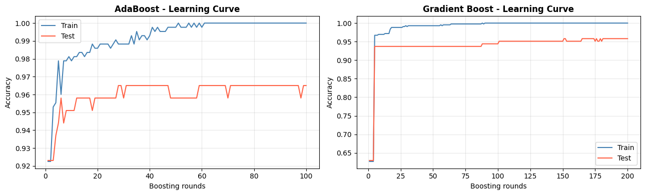
AdaBoost can overfit if run for too many rounds on noisy data. Gradient Boosting with a small learning rate tends to be more stable - the test curve levels off rather than degrades.