6.2.1.8. Boosting

All the ensemble methods on the Ensemble Methods page train their models in parallel and then average. Boosting is fundamentally different: models are trained sequentially, each one focused on correcting the mistakes of the ones before it.

The analogy is a student who reviews past exam papers: instead of preparing broadly, they prioritise the questions they got wrong last time. Each successive weak learner becomes progressively better at the hard cases.

This sequential correction means boosting reduces bias (the model becomes more accurate with each round), while parallel averaging primarily reduces variance. The cost is that boosting is more prone to overfitting if run for too many rounds.

Two algorithms dominate:

Algorithm	How the next model is targeted
AdaBoost	Re-weights training samples - hard samples get higher weight
Gradient Boosting	Fits the next model to the residuals (pseudo-gradients) of the current ensemble

---

AdaBoost

The Math

AdaBoost trains a sequence of weak learners \(h_1, h_2, \ldots, h_M\) (typically very shallow decision trees - “stumps”). After each step, training samples that were predicted incorrectly receive higher weights so the next learner focuses on them:

1. Initialise equal sample weights \(w_i = \frac{1}{n}\).

2. For \(m = 1, \ldots, M\):

   1. Train weak learner \(h_m\) on weighted samples.

   2. Compute weighted error: \(\varepsilon_m = \frac{\sum_i w_i \cdot \mathbf{1}[\text{error}_i > \tau]}{\sum_i w_i}\).

   3. Compute learner weight: \(\alpha_m = \frac{1}{2}\ln\!\frac{1-\varepsilon_m}{\varepsilon_m}\).

   4. Update sample weights: increase for hard samples, decrease for easy ones.

3. Final prediction: \(F(x) = \sum_{m=1}^{M} \alpha_m\, h_m(x)\).

The key difference from bagging: well-performing learners get higher \(\alpha_m\) and dominate the final vote.

---

Gradient Boosting

The Math

Gradient Boosting takes a more general view. It frames boosting as gradient descent in function space: at each step, fit a new weak learner \(h_m\) to the negative gradient of the loss with respect to the current prediction.

For MSE loss, the negative gradient is simply the residual \(y_i - F_{m-1}(x_i)\), so the update rule is:

\[F_m(x) = F_{m-1}(x) + \eta \cdot h_m(x)\]

where \(h_m\) is fitted to the residuals \(r_i = y_i - F_{m-1}(x_i)\) and \(\eta\) is the learning rate (called shrinkage).

Lower learning rates require more rounds but generally generalise better - the trade-off is controlled by learning_rate and n_estimators.

---

In scikit-learn

from sklearn.ensemble import AdaBoostRegressor, GradientBoostingRegressor

ada = AdaBoostRegressor(
    estimator=DecisionTreeRegressor(max_depth=3),
    n_estimators=100,
    learning_rate=0.1,
    random_state=42
)

gb = GradientBoostingRegressor(
    n_estimators=200,
    learning_rate=0.05,
    max_depth=3,
    random_state=42
)

Key hyperparameters:

Hyperparameter	Role
n_estimators	Number of boosting rounds - more can overfit
learning_rate	Shrinkage per round - lower → more rounds needed, better generalisation
max_depth	Depth of each weak learner - shallow trees (2–5) are standard
estimator (AdaBoost)	The weak learner type

---

Example

Show code cell source

Hide code cell source

import numpy as np
import pandas as pd
import matplotlib.pyplot as plt
from myst_nb import glue
from sklearn.ensemble import AdaBoostRegressor, GradientBoostingRegressor
from sklearn.tree import DecisionTreeRegressor
from sklearn.model_selection import train_test_split
from sklearn.metrics import mean_squared_error, r2_score
from sklearn.datasets import make_regression

np.random.seed(42)

X, y = make_regression(n_samples=300, n_features=10, n_informative=6,
                        noise=25, random_state=42)
X_train, X_test, y_train, y_test = train_test_split(
    X, y, test_size=0.25, random_state=42)

ada = AdaBoostRegressor(
    estimator=DecisionTreeRegressor(max_depth=3),
    n_estimators=100, learning_rate=0.1, random_state=42
)
gb = GradientBoostingRegressor(
    n_estimators=200, learning_rate=0.05, max_depth=3, random_state=42
)

ada.fit(X_train, y_train)
gb.fit(X_train, y_train)

for name, model in [("AdaBoost", ada), ("Gradient Boosting", gb)]:
    tr   = r2_score(y_train, model.predict(X_train))
    te   = r2_score(y_test,  model.predict(X_test))
    rmse = np.sqrt(mean_squared_error(y_test, model.predict(X_test)))
    print(f"{name:<22}  Train R²={tr:.3f}  Test R²={te:.3f}  RMSE={rmse:.1f}")

AdaBoost                Train R²=0.831  Test R²=0.646  RMSE=105.7
Gradient Boosting       Train R²=0.997  Test R²=0.838  RMSE=71.5

AdaBoost achieves test \(R^2\) = 0.646 (RMSE = 105.7). Gradient Boosting achieves 0.838 (RMSE = 71.5). Gradient Boosting generally outperforms AdaBoost because it can directly minimise the regression loss function.

Staged Learning Curves - When Does Overfitting Start?

Because boosting builds the model iteratively, we can inspect performance at every intermediate round - a powerful diagnostic:

Show code cell source

Hide code cell source

ada_train_staged, ada_test_staged = [], []
for yp_tr, yp_te in zip(ada.staged_predict(X_train), ada.staged_predict(X_test)):
    ada_train_staged.append(r2_score(y_train, yp_tr))
    ada_test_staged .append(r2_score(y_test,  yp_te))

gb_train_staged, gb_test_staged = [], []
for yp_tr, yp_te in zip(gb.staged_predict(X_train), gb.staged_predict(X_test)):
    gb_train_staged.append(r2_score(y_train, yp_tr))
    gb_test_staged .append(r2_score(y_test,  yp_te))

ada_best = int(np.argmax(ada_test_staged)) + 1
gb_best  = int(np.argmax(gb_test_staged))  + 1

fig, axes = plt.subplots(1, 2, figsize=(14, 4))

for ax, tr, te, best, title in [
    (axes[0], ada_train_staged, ada_test_staged, ada_best,
     "AdaBoost - Staged R²"),
    (axes[1], gb_train_staged,  gb_test_staged,  gb_best,
     "Gradient Boosting - Staged R²"),
]:
    rounds = np.arange(1, len(tr) + 1)
    ax.plot(rounds, tr, linewidth=2,   label="Train R²")
    ax.plot(rounds, te, linewidth=2,   linestyle="--", label="Test R²")
    ax.axvline(best, color="red", linestyle=":", linewidth=1.5,
               label=f"Best test round ({best})")
    ax.set_xlabel("Boosting Rounds", fontsize=12)
    ax.set_ylabel("R²", fontsize=12)
    ax.set_title(title, fontsize=12, fontweight="bold")
    ax.legend(fontsize=10)
    ax.grid(True, alpha=0.3)

plt.tight_layout()
plt.show()

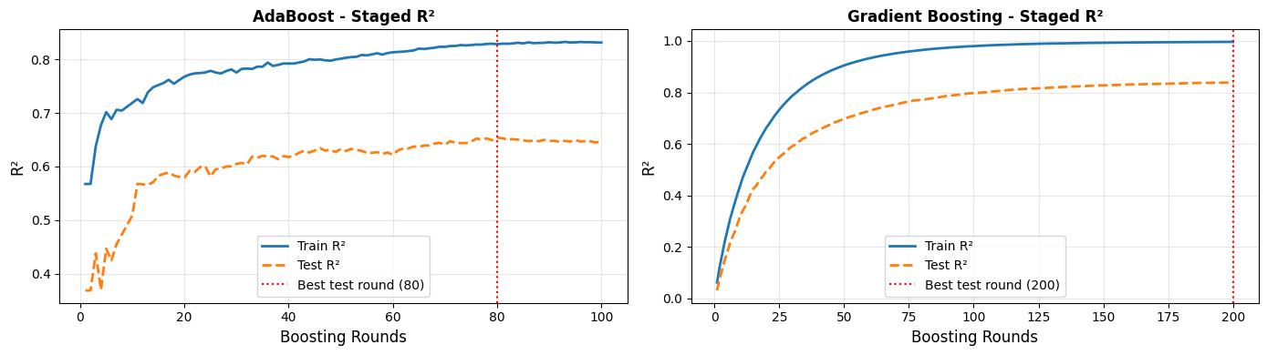
For AdaBoost, the best test performance is reached at round 80. Gradient Boosting peaks at round 200. Both eventually overfit if run for too many rounds - the staged learning curves make this visible and help you choose the right number of estimators.

Learning Rate vs Number of Estimators Trade-off

Show code cell source

Hide code cell source

configs = [
    (0.5, 50),
    (0.1, 200),
    (0.05, 400),
    (0.01, 1000),
]

rows = []
for lr, n in configs:
    m = GradientBoostingRegressor(n_estimators=n, learning_rate=lr,
                                   max_depth=3, random_state=42)
    m.fit(X_train, y_train)
    rows.append({
        "learning_rate": lr,
        "n_estimators":  n,
        "Train R²":      round(m.score(X_train, y_train), 3),
        "Test R²":       round(m.score(X_test,  y_test),  3),
    })

pd.DataFrame(rows)

	learning_rate	n_estimators	Train R²	Test R²
0	0.50	50	0.999	0.800
1	0.10	200	0.999	0.842
2	0.05	400	0.999	0.848
3	0.01	1000	0.997	0.837

Smaller learning rates with more rounds consistently match or beat larger learning rates - at the cost of training time. This is the standard shrinkage trade-off in boosting.

Prediction vs Ground Truth

Show code cell source

Hide code cell source

fig, axes = plt.subplots(1, 2, figsize=(12, 5))

for ax, model, title in [
    (axes[0], ada, f"AdaBoost  (R²={ada_test_r2})"),
    (axes[1], gb,  f"Gradient Boosting  (R²={gb_test_r2})"),
]:
    y_pred = model.predict(X_test)
    ax.scatter(y_test, y_pred, alpha=0.5, edgecolors="k", linewidths=0.3,
               color="steelblue")
    lo, hi = min(y_test.min(), y_pred.min()), max(y_test.max(), y_pred.max())
    ax.plot([lo, hi], [lo, hi], "r--", linewidth=1.5, label="Perfect prediction")
    ax.set_xlabel("True y", fontsize=11)
    ax.set_ylabel("Predicted y", fontsize=11)
    ax.set_title(title, fontsize=12, fontweight="bold")
    ax.legend(fontsize=10)
    ax.grid(True, alpha=0.3)

plt.tight_layout()
plt.show()

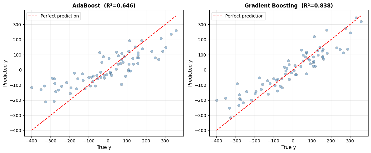
Points clustering tightly around the diagonal indicate accurate predictions. Gradient Boosting’s tighter cluster reflects its higher \(R^2\).

---

Strengths and Weaknesses

Strengths	Often achieves top performance on tabular data; reduces bias with each round; staged predictions make overfitting transparent
Weaknesses	Sequential training is slower than Random Forest; more hyperparameters to tune; sensitive to outliers (especially AdaBoost)

Tip

For most competitions and production settings, Gradient Boosting (or its optimised variants XGBoost, LightGBM, CatBoost) is the strongest off-the-shelf regressor. Start with learning_rate=0.05 and tune n_estimators using early stopping on a validation set.