6.2.1.5. Decision Tree Regression#
A decision tree makes predictions by asking a series of yes/no questions about the input features, following a flowchart from the root to a leaf node. At every internal node the tree asks: “Is feature \(j\) above threshold \(t\)?” It routes the sample left or right, and the process repeats until a leaf is reached. The prediction at that leaf is the mean of all training targets that fell into the same region.
Think of it as partitioning the feature space into axis-aligned rectangles. Each rectangle gets one constant prediction - the average of the training points inside it.
Unlike linear models, a decision tree can capture any non-linear relationship without feature engineering. This power comes at a cost: deep trees memorise the training data perfectly but generalise poorly - the classic variance problem. Controlling tree depth is therefore the central challenge.
The Math#
At each node the algorithm searches over all features \(j\) and all possible thresholds \(t\) to find the split that most reduces the MSE over the training samples in that node:
The prediction at a leaf containing region \(\mathcal{R}_m\) is:
Key hyperparameters:
Hyperparameter |
Effect |
|---|---|
|
Maximum levels of splits - primary control over complexity |
|
Minimum training samples per leaf - higher → smoother model |
|
Minimum samples required to attempt any split |
|
Number of features considered at each split |
In scikit-learn#
from sklearn.tree import DecisionTreeRegressor

tree = DecisionTreeRegressor(max_depth=5, min_samples_leaf=5, random_state=42)
tree.fit(X_train, y_train)
No feature scaling is required - trees split on rank-order, not magnitude.
Example#
tree = DecisionTreeRegressor(max_depth=5, random_state=42)
tree.fit(X_train, y_train)

train_r2  = r2_score(y_train, tree.predict(X_train))
test_r2   = r2_score(y_test,  tree.predict(X_test))
test_rmse = np.sqrt(mean_squared_error(y_test, tree.predict(X_test)))

print(f"Train R²  : {train_r2:.3f}")
print(f"Test  R²  : {test_r2:.3f}")
print(f"Test  RMSE: {test_rmse:.1f}")
Train R²  : 0.882
Test  R²  : 0.300
Test  RMSE: 148.7
With max_depth=5 the tree achieves a test \(R^2\) of 0.3 and RMSE of 148.7. Train \(R^2\) of 0.882 is notably higher, signalling some overfitting - this is typical of decision trees.
Visualising the Tree Structure#
scikit-learn’s plot_tree renders the full decision flowchart. A max_depth=3 tree is used here so the diagram stays readable - each node shows the split rule, the MSE at that node, the number of samples, and the predicted value.
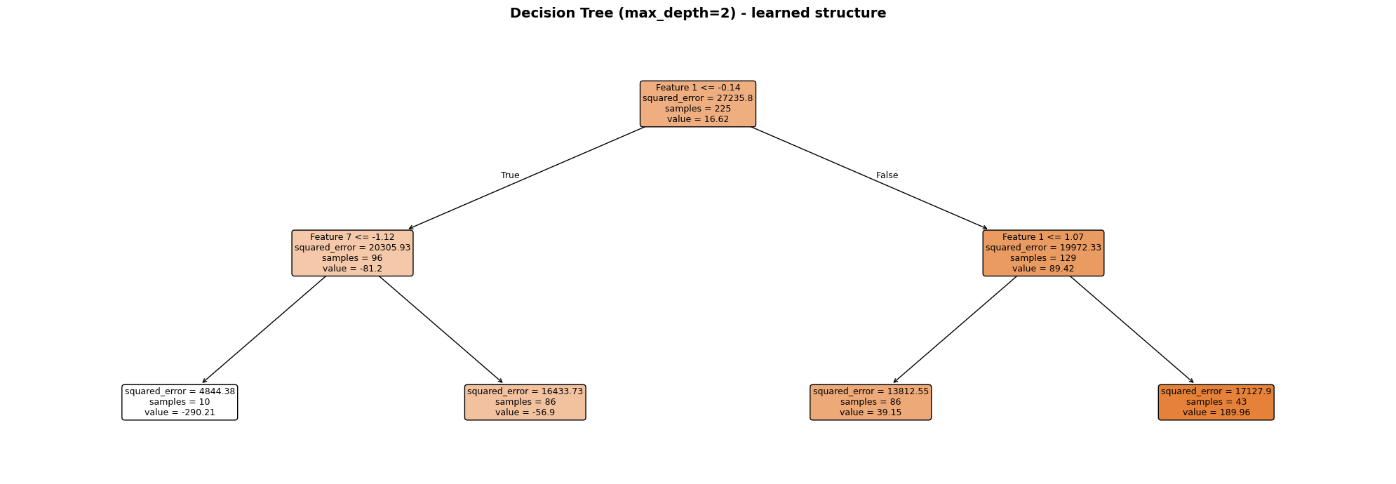
Each node is colour-coded by its mean prediction (darker = higher value). The root split always uses the single most informative feature; subsequent splits refine the prediction in each sub-region. Leaf nodes display the constant prediction that will be returned for any sample that reaches them.
The Bias–Variance Trade-off Across Depths#
depths = [1, 2, 3, 5, 8, 12, None]

rows = []
for d in depths:
    m = DecisionTreeRegressor(max_depth=d, random_state=42)
    m.fit(X_train, y_train)
    rows.append({
        "max_depth":   str(d),
        "Train R²":    round(r2_score(y_train, m.predict(X_train)), 3),
        "Test R²":     round(r2_score(y_test,  m.predict(X_test)),  3),
        "Test RMSE":   round(np.sqrt(mean_squared_error(y_test, m.predict(X_test))), 1),
    })

depth_df = pd.DataFrame(rows)
depth_df
| max_depth | Train R² | Test R² | Test RMSE | |
|---|---|---|---|---|
| 0 | 1 | 0.261 | 0.102 | 168.6 |
| 1 | 2 | 0.447 | 0.090 | 169.7 |
| 2 | 3 | 0.626 | 0.347 | 143.7 |
| 3 | 5 | 0.882 | 0.300 | 148.7 |
| 4 | 8 | 0.988 | 0.445 | 132.4 |
| 5 | 12 | 1.000 | 0.464 | 130.2 |
| 6 | None | 1.000 | 0.475 | 128.9 |
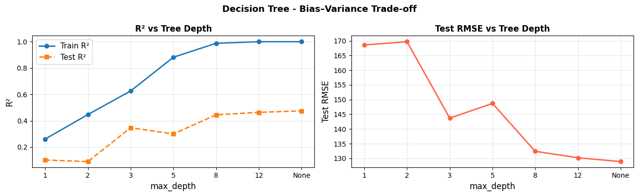
As depth increases, training error falls toward zero (the tree memorises the data) while test error first decreases, then rises again. The sweet spot is usually somewhere in the middle - here around max_depth=5.
Visualising Splits on 1-D Data#
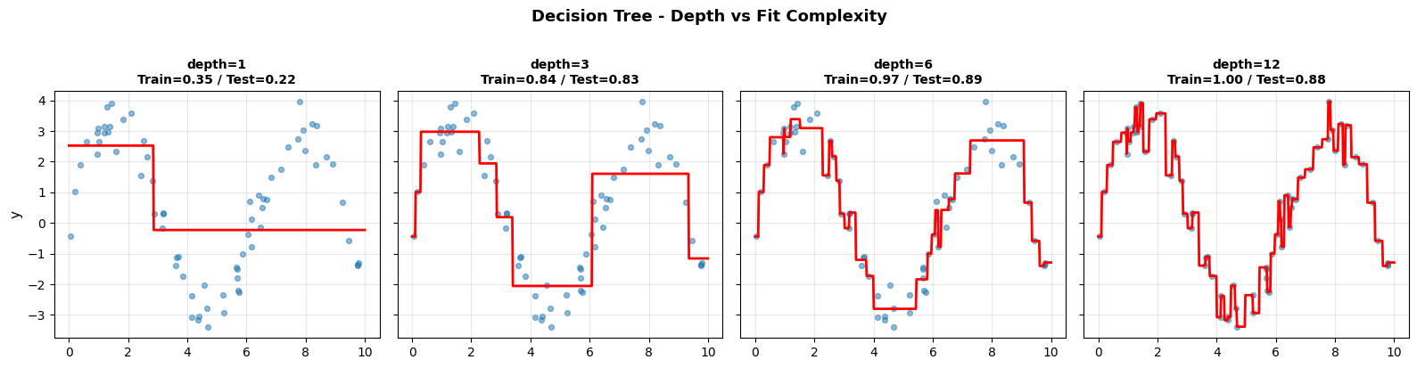
The step-function predictions are clearly visible: shallow trees produce coarse approximations (high bias), while deep trees follow every wiggle in the training data (high variance).
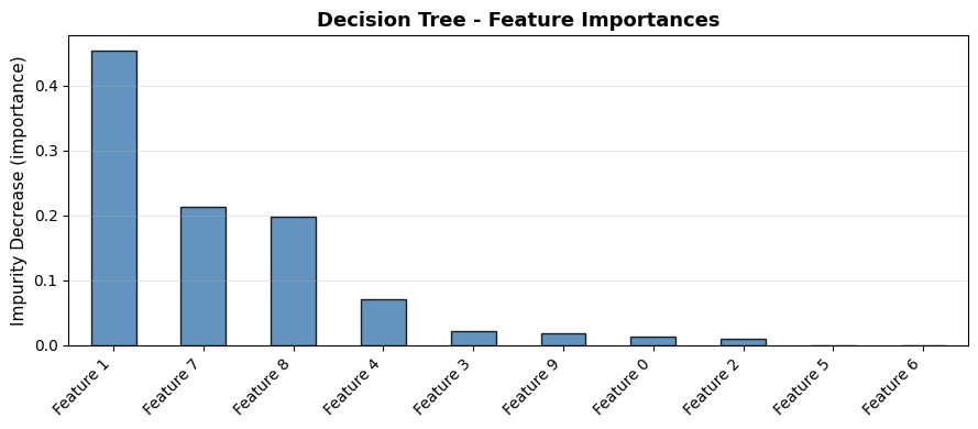
Feature Importance#
Strengths and Weaknesses#
Strengths |
No feature scaling needed; handles non-linearity; interpretable (visualise the tree); mixed feature types |
Weaknesses |
High variance - sensitive to small data changes; prone to overfitting at large depths |
Tip
Single decision trees are rarely used in isolation for competitive performance. They are the core building block for Random Forest (bagging) and Boosting (boosting) - ensemble methods that correct their variance problem.