6.3.1.2. Hierarchical Clustering

K-Means forces you to choose the number of clusters before you see the data. Hierarchical clustering takes a different approach: it builds a complete tree of groupings — from each point in its own cluster all the way up to one single cluster — and lets you decide where to cut.

The result is a dendrogram: a tree diagram that shows, at a glance, how similar groups merge and at what scale structure appears. This makes hierarchical clustering the preferred tool when you want to explore your data before committing to a particular \(k\).

---

The Intuition

The most common variant is agglomerative (bottom-up) clustering:

1. Start with \(n\) clusters — one per data point.

2. Find the two closest clusters.

3. Merge them into a single cluster.

4. Repeat steps 2–3 until one cluster remains.

At each step the algorithm records which clusters merged and at what distance. That history is the dendrogram. To obtain any desired number of clusters, you simply draw a horizontal line across the dendrogram and count how many vertical lines it cuts.

---

The Math

The one degree of freedom is how you measure the distance between two clusters (not individual points). This is the linkage criterion:

Linkage	Distance between clusters \(A\) and \(B\)	Behaviour
Single	\(\min_{a \in A, b \in B} d(a, b)\)	Chaining effect; finds elongated clusters
Complete	\(\max_{a \in A, b \in B} d(a, b)\)	Compact clusters; sensitive to outliers
Average	$\frac{1}{	A
Ward	Increase in total WCSS after merge	Minimises variance; produces similar-sized clusters

Ward’s linkage is usually the best default. It produces compact, similarly-sized clusters and aligns most closely with K-Means’ objective.

The agglomerative process has time complexity \(O(n^2 \log n)\) and space complexity \(O(n^2)\), making it impractical for very large datasets (> ~10 000 points).

---

In scikit-learn

from sklearn.cluster import AgglomerativeClustering

model = AgglomerativeClustering(n_clusters=3, linkage='ward')
labels = model.fit_predict(X_sc)

To visualise the dendrogram, use scipy:

from scipy.cluster.hierarchy import dendrogram, linkage

Z = linkage(X_sc, method='ward')
dendrogram(Z)

Key parameters:

Parameter	Meaning
n_clusters	Number of clusters to cut the tree at
linkage	'ward', 'complete', 'average', 'single'
metric	Distance metric (default 'euclidean'; not used with 'ward')

---

Example

Show code cell source

Hide code cell source

import numpy as np
import pandas as pd
import matplotlib.pyplot as plt
from sklearn.cluster import AgglomerativeClustering
from sklearn.datasets import load_iris
from sklearn.preprocessing import StandardScaler
from scipy.cluster.hierarchy import dendrogram, linkage

np.random.seed(42)

data   = load_iris()
X, y   = data.data, data.target
scaler = StandardScaler()
X_sc   = scaler.fit_transform(X)

Reading the Dendrogram

Z = linkage(X_sc, method='ward')

fig, ax = plt.subplots(figsize=(14, 5))
dendrogram(Z, ax=ax, truncate_mode='lastp', p=20,
           leaf_rotation=45, leaf_font_size=10,
           color_threshold=6.5, above_threshold_color='grey')
ax.axhline(y=6.5, color='tomato', linestyle='--', linewidth=1.5, label='Cut at 3 clusters')
ax.set_xlabel('Sample index (or cluster size)', fontsize=12)
ax.set_ylabel('Ward distance', fontsize=12)
ax.set_title('Dendrogram — Iris Dataset (Ward linkage)', fontsize=13, fontweight='bold')
ax.legend()
ax.grid(True, alpha=0.3, axis='y')
plt.tight_layout()
plt.show()

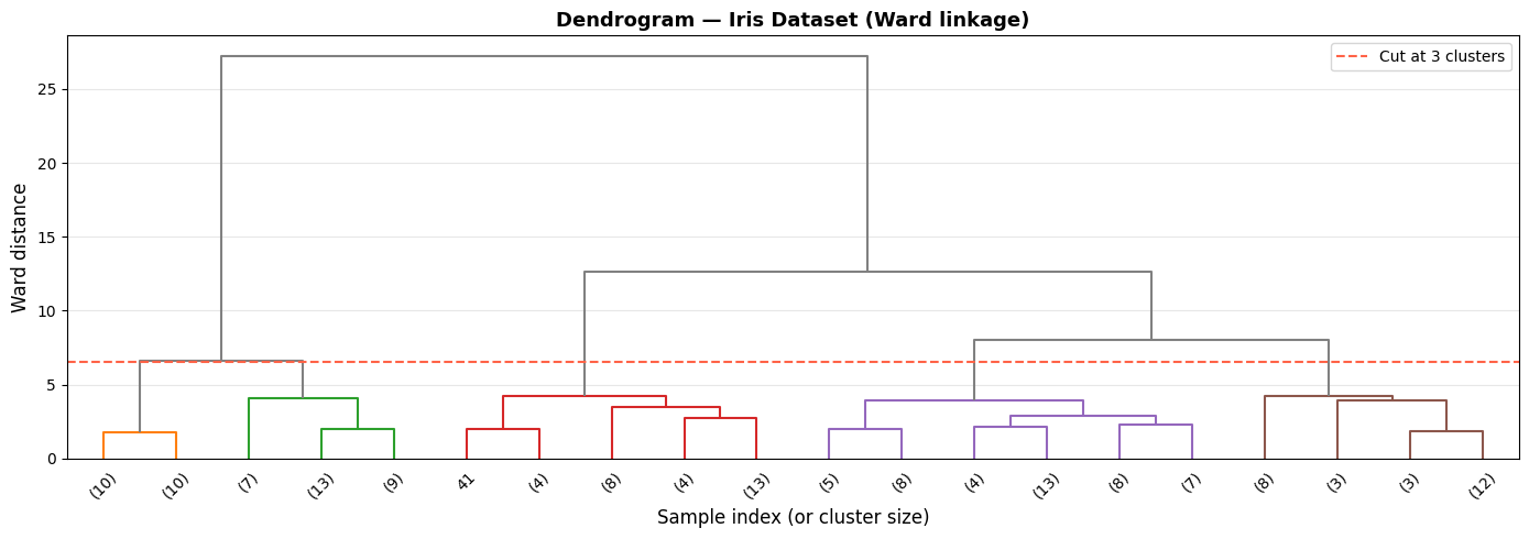
The dendrogram shows a clear split into three main branches. The large vertical jump just below the red line tells us the three-cluster solution has exceptionally high between-cluster distance — exactly where you want to cut.

Fitted Clusters vs True Labels

from sklearn.decomposition import PCA

model = AgglomerativeClustering(n_clusters=3, linkage='ward')
labels_pred = model.fit_predict(X_sc)

pca  = PCA(n_components=2)
X_2d = pca.fit_transform(X_sc)

fig, axes = plt.subplots(1, 2, figsize=(13, 5))
titles      = ['Agglomerative Clusters (predicted)', 'True Iris Species']
label_sets  = [labels_pred, y]
class_names = [['Cluster 0', 'Cluster 1', 'Cluster 2'], data.target_names.tolist()]

for ax, labs, title, names in zip(axes, label_sets, titles, class_names):
    for cls in np.unique(labs):
        mask = labs == cls
        ax.scatter(X_2d[mask, 0], X_2d[mask, 1],
                   label=names[cls], alpha=0.75, edgecolors='k', linewidths=0.3, s=55)
    ax.set_xlabel('PC 1', fontsize=11)
    ax.set_ylabel('PC 2', fontsize=11)
    ax.set_title(title, fontsize=12, fontweight='bold')
    ax.legend(fontsize=9)
    ax.grid(True, alpha=0.3)

plt.suptitle('Hierarchical Clustering on Iris (2-D PCA projection)', fontsize=14, fontweight='bold')
plt.tight_layout()
plt.show()

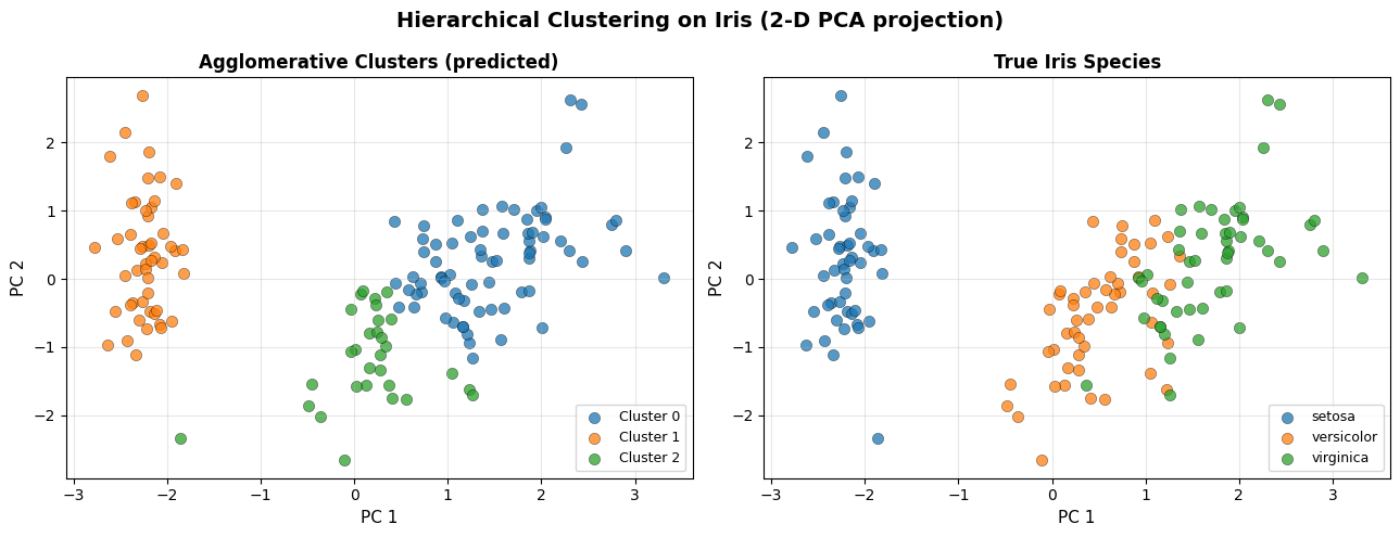
Ward linkage cleanly separates setosa from the other two species and draws a reasonable boundary between versicolor and virginica — without ever being told the labels.

Effect of Linkage Criteria

linkages  = ['ward', 'complete', 'average', 'single']
fig, axes = plt.subplots(1, 4, figsize=(18, 4))

for ax, lnk in zip(axes, linkages):
    try:
        m = AgglomerativeClustering(n_clusters=3, linkage=lnk)
        lbl = m.fit_predict(X_sc)
    except Exception:
        ax.set_title(f'{lnk}\n(incompatible)', fontsize=11)
        continue
    for cls in np.unique(lbl):
        mask = lbl == cls
        ax.scatter(X_2d[mask, 0], X_2d[mask, 1], alpha=0.75,
                   edgecolors='k', linewidths=0.3, s=45)
    ax.set_title(f'Linkage: {lnk}', fontsize=11, fontweight='bold')
    ax.set_xlabel('PC 1'); ax.set_ylabel('PC 2')
    ax.grid(True, alpha=0.3)

plt.suptitle('Iris — Effect of Linkage Criteria', fontsize=14, fontweight='bold')
plt.tight_layout()
plt.show()

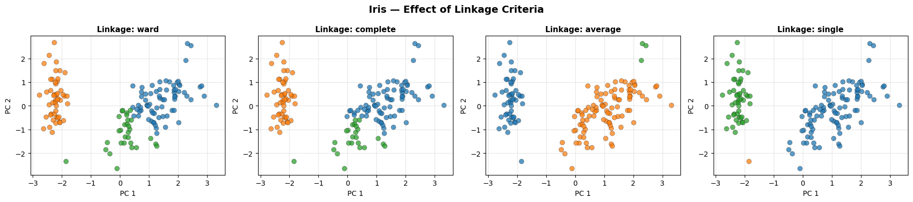
Ward and complete linkage produce the most compact, well-separated clusters. Single linkage suffers from the chaining effect, where a string of close points merges two large groups prematurely.

---

Strengths and Weaknesses

Strengths	No need to pre-specify \(k\); dendrogram reveals structure at every scale; deterministic (no random initialisation)
Weaknesses	\(O(n^2)\) memory — impractical for large datasets; merges are irreversible (greedy); sensitive to noise and outliers

Tip

Use the dendrogram to choose \(k\) by looking for the largest vertical gap before the first horizontal line crossing the cut threshold. That gap indicates a stable, well-separated partition.