6.2.2.4. Naïve Bayes#
Naïve Bayes is a generative probabilistic classifier rooted in Bayes’ theorem. It models the joint distribution of features and class labels, then inverts it to obtain class probabilities. The “naïve” part refers to its key assumption: all features are conditionally independent given the class label.
This assumption is almost always violated in practice - pixel intensities in an image, or words in a document, are obviously correlated. Yet Naïve Bayes is surprisingly competitive, particularly for text classification, and has compelling practical virtues:
Extremely fast to train (\(O(n \cdot p)\), closed-form parameter estimates)
Works well with very little data
Naturally handles multi-class problems
Produces well-calibrated probability estimates
In contrast to discriminative models like Logistic Regression, Naïve Bayes explicitly models how each class generates its features.
The Math#
Bayes’ theorem gives us the posterior class probability:
Since \(P(\mathbf{x})\) is the same for all classes, we need only the numerator:
The naïve independence assumption turns the joint likelihood into a product of univariate terms, which is tractable to estimate.
Gaussian Naïve Bayes assumes each feature is normally distributed within each class:
Parameters \(\mu_{cj}\) and \(\sigma_{cj}^2\) are estimated as the per-class feature sample mean and variance - no optimisation loop required.
Variants by feature type:
Variant |
Designed for |
|---|---|
|
Continuous features (assumes Gaussian within each class) |
|
Count data (word counts in text) |
|
Binary features (word presence/absence) |
|
Imbalanced text classification |
In scikit-learn#
from sklearn.naive_bayes import GaussianNB

gnb = GaussianNB(var_smoothing=1e-9)  # add small constant to variances for stability
gnb.fit(X_train, y_train)
y_pred = gnb.predict(X_test)
y_prob = gnb.predict_proba(X_test)[:, 1]
Gaussian NB does not require feature scaling - it models each feature’s distribution independently. The only hyperparameter is var_smoothing, which prevents zero-variance issues for features that are constant within a class.
Example#
from sklearn.naive_bayes import GaussianNB

gnb = GaussianNB()
gnb.fit(X_train, y_train)

train_acc = accuracy_score(y_train, gnb.predict(X_train))
test_acc  = accuracy_score(y_test,  gnb.predict(X_test))
test_auc  = roc_auc_score(y_test,   gnb.predict_proba(X_test)[:, 1])
Gaussian Naïve Bayes achieves a test accuracy of 0.937 and AUC-ROC of 0.989 - competitive despite the strong independence assumption. Train accuracy of 0.946 confirms the model is not overfitting.
Class-Conditional Feature Distributions#
Because Naïve Bayes is a generative model, we can inspect the estimated per-class Gaussian distributions and see which features best separate the two classes.
feature_indices = [0, 2, 20, 22]   # mean radius, mean perimeter, worst radius, worst perimeter
feature_names   = data.feature_names

fig, axes = plt.subplots(1, len(feature_indices), figsize=(14, 4))

for ax, fi in zip(axes, feature_indices):
    for ci, (label, color) in enumerate(zip(data.target_names, ['tomato', 'steelblue'])):
        mu    = gnb.theta_[ci, fi]
        sigma = np.sqrt(gnb.var_[ci, fi])
        xs    = np.linspace(mu - 4*sigma, mu + 4*sigma, 200)
        ax.plot(xs, 1/(sigma*np.sqrt(2*np.pi)) * np.exp(-0.5*((xs-mu)/sigma)**2),
                color=color, lw=2, label=label)
    ax.set_title(feature_names[fi], fontsize=9, fontweight='bold')
    ax.set_yticks([])
    ax.legend(fontsize=7)
    ax.grid(True, alpha=0.3)

fig.suptitle("Estimated Class-Conditional Feature Distributions",
             fontweight='bold', y=1.01)
plt.tight_layout()
plt.show()
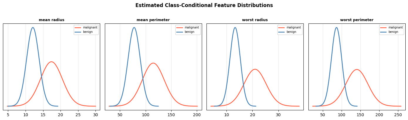
Features with well-separated class distributions (little overlap) contribute most to correct classification.