6.3.2.3. UMAP: Uniform Manifold Approximation and Projection#
t-SNE produces beautiful cluster visualisations but comes with a practical cost: it is slow, non-deterministic, cannot project new points without re-fitting, and discards global structure. UMAP, published in 2018, addresses all four limitations simultaneously.
UMAP is grounded in Riemannian geometry and algebraic topology, but its practical behaviour is easy to summarise: it builds a graph that captures the local neighbourhood structure of the data, then finds a low-dimensional layout that preserves that graph as faithfully as possible — while also keeping large-scale structure intact far better than t-SNE.
In practice, UMAP is:
Much faster — typically 10–100× quicker than t-SNE on the same dataset.
More consistent — largely deterministic across runs (with a fixed seed).
Better at global structure — the relative positions of clusters carry more meaning.
Versatile — supports out-of-sample projection, making it usable inside ML pipelines.
The Intuition#
UMAP proceeds in two stages:
Graph construction — build a fuzzy, weighted nearest-neighbour graph in the high-dimensional space. Each edge weight reflects how confident we are that two points are truly neighbours (it falls off smoothly with distance, and is calibrated so that each point has a roughly equal “local scale”).
Layout optimisation — find a low-dimensional embedding that minimises the cross-entropy between the high-D fuzzy graph and a similarly constructed low-D graph. This is done via stochastic gradient descent, which is far faster than t-SNE’s force-directed approach.
The “fuzzy” definition of the graph is what allows UMAP to handle manifolds of varying density intelligently — a common failure mode for t-SNE.
The Math (at a glance)#
For each point \(\mathbf{x}_i\) and its \(k\)-nearest neighbour \(\mathbf{x}_{j}\), define a membership strength:
where \(\rho_i\) is the distance to the nearest neighbour (ensures continuity of the manifold) and \(\sigma_i\) is calibrated to achieve a target “effective connectivity” of \(\log_2 k\).
The symmetrised graph weight is:
In the low-D space, membership is modelled with a smooth family of curves:
The parameters \(a\) and \(b\) are determined by min_dist. The embedding is optimised by minimising the binary cross-entropy:
In practice#
# Install: pip install umap-learn
import umap

reducer = umap.UMAP(n_components=2, n_neighbors=15, min_dist=0.1, random_state=42)
X_umap  = reducer.fit_transform(X_sc)

# Out-of-sample projection (unlike t-SNE, this works!)
X_new_umap = reducer.transform(X_new_sc)
Key parameters:
Parameter |
Meaning |
|---|---|
|
Size of local neighbourhood; small → fine local structure; large → more global |
|
Minimum distance between points in the embedding; small → tighter clusters |
|
Output dimensionality (2 for visualisation; higher for pre-processing) |
|
Distance metric ( |
Example#
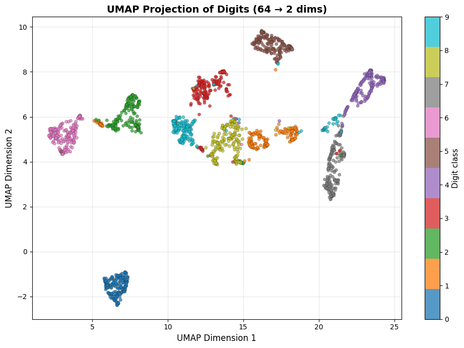
UMAP on the Digits Dataset#
import time
t0 = time.time()
reducer = umap_lib.UMAP(n_components=2, n_neighbors=15,
                        min_dist=0.1, random_state=42)
X_umap = reducer.fit_transform(X_sc)
print(f"UMAP runtime: {time.time() - t0:.1f} s")

fig, ax = plt.subplots(figsize=(10, 7))
sc = ax.scatter(X_umap[:, 0], X_umap[:, 1],
                c=y, cmap='tab10', alpha=0.75,
                edgecolors='k', linewidths=0.2, s=20)
cbar = plt.colorbar(sc, ax=ax, ticks=range(10))
cbar.set_label('Digit class', fontsize=11)
ax.set_xlabel('UMAP Dimension 1', fontsize=12)
ax.set_ylabel('UMAP Dimension 2', fontsize=12)
ax.set_title('UMAP Projection of Digits (64 → 2 dims)',
                fontsize=14, fontweight='bold')
ax.grid(True, alpha=0.3)
plt.tight_layout()
plt.show()
/home/runner/work/datasciencethenovel/datasciencethenovel/.venv/lib/python3.13/site-packages/umap/umap_.py:1952: UserWarning: n_jobs value 1 overridden to 1 by setting random_state. Use no seed for parallelism.
  warn(
UMAP runtime: 10.6 s
Effect of n_neighbors#
neighbor_vals = [5, 15, 50]
fig, axes = plt.subplots(1, 3, figsize=(18, 5))

for ax, nn in zip(axes, neighbor_vals):
    emb = umap_lib.UMAP(n_components=2, n_neighbors=nn,
                        min_dist=0.1, random_state=42).fit_transform(X_sc)
    ax.scatter(emb[:, 0], emb[:, 1], c=y, cmap='tab10',
                alpha=0.65, edgecolors='k', linewidths=0.15, s=16)
    ax.set_title(f'n_neighbors = {nn}', fontsize=12, fontweight='bold')
    ax.set_xticks([]); ax.set_yticks([])
    ax.grid(True, alpha=0.2)

plt.suptitle('UMAP n_neighbors Sensitivity — Digits Dataset',
                fontsize=14, fontweight='bold')
plt.tight_layout()
plt.show()
/home/runner/work/datasciencethenovel/datasciencethenovel/.venv/lib/python3.13/site-packages/umap/umap_.py:1952: UserWarning: n_jobs value 1 overridden to 1 by setting random_state. Use no seed for parallelism.
  warn(
/home/runner/work/datasciencethenovel/datasciencethenovel/.venv/lib/python3.13/site-packages/umap/umap_.py:1952: UserWarning: n_jobs value 1 overridden to 1 by setting random_state. Use no seed for parallelism.
  warn(
/home/runner/work/datasciencethenovel/datasciencethenovel/.venv/lib/python3.13/site-packages/umap/umap_.py:1952: UserWarning: n_jobs value 1 overridden to 1 by setting random_state. Use no seed for parallelism.
  warn(
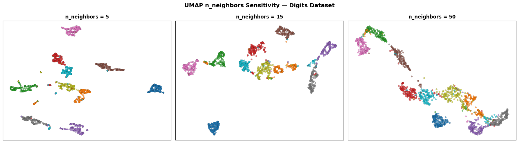
Small n_neighbors emphasises fine local clusters at the cost of global coherence. Large n_neighbors produces a more continuous landscape where the relative positions of digit classes become visible — something t-SNE rarely achieves.
Strengths and Weaknesses#
Strengths |
Much faster than t-SNE; preserves global structure; supports out-of-sample projection; largely deterministic; works with non-Euclidean metrics |
Weaknesses |
External dependency ( |
Tip
UMAP is the preferred choice when you need a visualisation tool you can reuse (i.e., project new points onto an existing layout), or when your dataset is large enough that t-SNE’s \(O(n^2)\) cost is prohibitive.