6.2.3.2. Optimizers

The perceptron’s simple update rule works only for linearly separable data. For neural networks - with non-linear activations, many layers, and a non-convex loss landscape - we need a general-purpose learning algorithm: gradient descent.

An optimizer implements a strategy for using the gradient of the loss to update the network weights at each step. Choosing the right optimizer (and learning rate) is one of the most important practical decisions when training a neural network.

---

The Core Idea

The loss function \(\mathcal{L}(\mathbf{w})\) measures how wrong the current weights are. The gradient \(\nabla_\mathbf{w}\mathcal{L}\) tells us the direction of steepest ascent in weight space. To reduce the loss, we step in the opposite direction:

Key intuition: Imagine standing on a hilly landscape in fog. You cannot see the valley, but you can feel the slope under your feet. To reach the lowest point, always step downhill.

The challenge is choosing how big each step should be, and whether to look at the entire terrain (all data) or just one footstep (one sample) before deciding where to go next.

---

The Math

Gradient Descent (Full Batch)

Compute the gradient over the entire training set, then update once:

\[\mathbf{w} \leftarrow \mathbf{w} - \eta\,\nabla_\mathbf{w}\mathcal{L}(\mathbf{w})\]

where \(\eta\) is the learning rate. Stable and smooth, but each update requires a full pass over \(n\) examples - too slow for large datasets.

Stochastic Gradient Descent (SGD)

Compute the gradient from a single randomly chosen example, then update:

\[\mathbf{w} \leftarrow \mathbf{w} - \eta\,\nabla_\mathbf{w}\mathcal{L}(\mathbf{w};\, \mathbf{x}_i, y_i)\]

Updates are noisy (one sample is not representative of the full dataset), but this noise can actually help escape shallow local minima. Crucially, it is fast: one weight update takes \(O(p)\) work regardless of \(n\).

Mini-Batch SGD

The practical standard: use a small random batch of \(m\) examples (typically 32–512) per update. Balances the stability of full-batch and the speed of SGD:

\[\mathbf{w} \leftarrow \mathbf{w} - \eta\,\frac{1}{m}\sum_{i \in \mathcal{B}}\nabla_\mathbf{w}\mathcal{L}(\mathbf{w};\,\mathbf{x}_i, y_i)\]

---

Advanced Optimizers

Plain SGD treats every weight and every direction equally. Modern optimizers adaptively scale the learning rate to converge faster and more reliably.

SGD with Momentum

Momentum accumulates a velocity vector \(\mathbf{v}\) in directions of persistent gradient, reducing oscillations:

\[\mathbf{v} \leftarrow \beta\,\mathbf{v} - \eta\,\nabla\mathcal{L} \qquad \mathbf{w} \leftarrow \mathbf{w} + \mathbf{v}\]

Typical momentum coefficient: \(\beta = 0.9\).

RMSProp

Divides the learning rate by a moving average of squared gradients, so parameters with large recent gradients get smaller updates:

\[s_j \leftarrow \beta\,s_j + (1-\beta)\,\left(\frac{\partial \mathcal{L}}{\partial w_j}\right)^2 \qquad w_j \leftarrow w_j - \frac{\eta}{\sqrt{s_j + \varepsilon}}\cdot \frac{\partial\mathcal{L}}{\partial w_j}\]

Good for non-stationary problems and recurrent networks.

Adam (Adaptive Moment Estimation)

Adam combines the ideas of momentum (first moment) and RMSProp (second moment) with bias correction for the early steps:

\[m_j \leftarrow \beta_1 m_j + (1-\beta_1)\,g_j \qquad v_j \leftarrow \beta_2 v_j + (1-\beta_2)\,g_j^2\]

\[\hat{m}_j = \frac{m_j}{1-\beta_1^t} \quad \hat{v}_j = \frac{v_j}{1-\beta_2^t} \qquad w_j \leftarrow w_j - \frac{\eta}{\sqrt{\hat{v}_j}+\varepsilon}\,\hat{m}_j\]

Default parameters: \(\beta_1=0.9\), \(\beta_2=0.999\), \(\varepsilon=10^{-8}\).

Adam is the most popular default for deep learning: it converges quickly, requires little learning-rate tuning, and works well across diverse architectures.

Quick comparison:

Optimizer	Convergence	Tuning effort	Best for
SGD	Slow, noisy	Learning rate + schedule	Convex problems, fine-tuning
SGD + Momentum	Faster	\(\eta\), \(\beta\)	General deep learning
RMSProp	Fast	\(\eta\), \(\beta\)	RNNs, non-stationary
Adam	Fast	Usually \(\eta\) only	Default choice

---

In scikit-learn

MLPClassifier and MLPRegressor expose optimizers through the solver parameter:

from sklearn.neural_network import MLPClassifier

# SGD
mlp_sgd = MLPClassifier(solver='sgd', learning_rate_init=0.01,
                         momentum=0.9, max_iter=200, random_state=42)

# Adam (default and recommended)
mlp_adam = MLPClassifier(solver='adam', learning_rate_init=0.001,
                          max_iter=200, random_state=42)

# L-BFGS (full-batch quasi-Newton, good for small datasets)
mlp_lbfgs = MLPClassifier(solver='lbfgs', max_iter=1000, random_state=42)

The loss_curve_ attribute records the training loss at each iteration, allowing you to diagnose convergence issues.

---

Example

Show code cell source

Hide code cell source

import numpy as np
import pandas as pd
import matplotlib.pyplot as plt
from myst_nb import glue
from sklearn.neural_network import MLPClassifier
from sklearn.datasets import load_digits
from sklearn.model_selection import train_test_split
from sklearn.preprocessing import StandardScaler
from sklearn.metrics import accuracy_score

np.random.seed(42)

# Shared dataset used throughout all Neural Network pages
data = load_digits()
X, y = data.data, data.target
X_train, X_test, y_train, y_test = train_test_split(
    X, y, test_size=0.25, random_state=42, stratify=y)

scaler = StandardScaler()
X_train_sc = scaler.fit_transform(X_train)
X_test_sc  = scaler.transform(X_test)

from sklearn.neural_network import MLPClassifier

solvers = {
    "SGD":   MLPClassifier(hidden_layer_sizes=(64,), solver='sgd',
                            learning_rate_init=0.01, momentum=0.9,
                            max_iter=300, random_state=42),
    "Adam":  MLPClassifier(hidden_layer_sizes=(64,), solver='adam',
                            learning_rate_init=0.001,
                            max_iter=300, random_state=42),
    "LBFGS": MLPClassifier(hidden_layer_sizes=(64,), solver='lbfgs',
                            max_iter=1000, random_state=42),
}

results = {}
for name, model in solvers.items():
    model.fit(X_train_sc, y_train)
    results[name] = {
        "Train Acc": round(accuracy_score(y_train, model.predict(X_train_sc)), 3),
        "Test Acc":  round(accuracy_score(y_test,  model.predict(X_test_sc)),  3),
        "Iterations": model.n_iter_,
    }

pd.DataFrame(results).T

	Train Acc	Test Acc	Iterations
SGD	1.0	0.976	185.0
Adam	1.0	0.980	164.0
LBFGS	1.0	0.982	15.0

Convergence Curves

fig, ax = plt.subplots(figsize=(9, 4))

colors = ['steelblue', 'tomato', 'seagreen']
for (name, model), color in zip(solvers.items(), colors):
    if hasattr(model, 'loss_curve_'):
        ax.plot(model.loss_curve_, label=name, color=color, lw=2)

ax.set_xlabel("Iterations")
ax.set_ylabel("Training Loss")
ax.set_title("Optimizer Convergence -  Digits Dataset (single hidden layer, 64 units)",
             fontweight='bold')
ax.legend()
ax.grid(True, alpha=0.3)
plt.tight_layout()
plt.show()

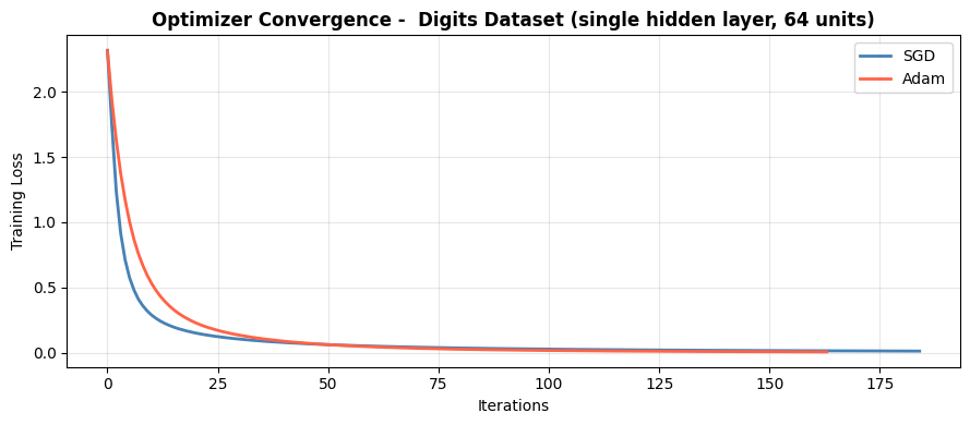
Adam converges smoothly and reaches a test accuracy of 0.98. SGD converges more slowly and noisily with the same learning rate - adding a learning rate schedule or using a larger initial rate would close the gap. L-BFGS converges in one batch pass (no loss curve) and can be very effective on small-to-medium datasets.

Learning Rate Sensitivity

The learning rate is the most important hyperparameter for SGD. Too large → divergence; too small → very slow convergence.

lrs = [0.1, 0.01, 0.001, 0.0001]
fig, axes = plt.subplots(1, len(lrs), figsize=(14, 3.5), sharey=True)

for ax, lr in zip(axes, lrs):
    m = MLPClassifier(hidden_layer_sizes=(64,), solver='sgd',
                      learning_rate_init=lr, max_iter=300, random_state=42)
    m.fit(X_train_sc, y_train)
    ax.plot(m.loss_curve_, color='steelblue', lw=1.5)
    ax.set_title(f"lr = {lr}", fontweight='bold')
    ax.set_xlabel("Iterations")
    if ax is axes[0]:
        ax.set_ylabel("Training Loss")
    ax.grid(True, alpha=0.3)

plt.suptitle("SGD -  Effect of Learning Rate", fontweight='bold', y=1.02)
plt.tight_layout()
plt.show()

/home/runner/work/datasciencethenovel/datasciencethenovel/.venv/lib/python3.13/site-packages/sklearn/neural_network/_multilayer_perceptron.py:781: ConvergenceWarning: Stochastic Optimizer: Maximum iterations (300) reached and the optimization hasn't converged yet.
  warnings.warn(

/home/runner/work/datasciencethenovel/datasciencethenovel/.venv/lib/python3.13/site-packages/sklearn/neural_network/_multilayer_perceptron.py:781: ConvergenceWarning: Stochastic Optimizer: Maximum iterations (300) reached and the optimization hasn't converged yet.
  warnings.warn(

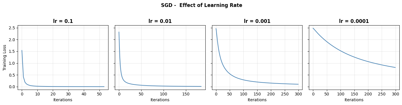
A learning rate of 0.01 converges well here. 0.1 may diverge or oscillate; 0.0001 makes very slow progress. Adam is far less sensitive to this choice, which is why it is the practical default.