6.1.7. Regularization: Taming Complexity

In the previous sections, we explored overfitting and the bias–variance tradeoff. We saw how models that are too flexible can memorize noise instead of learning structure. Regularization is the natural next step. It provides a principled way to control complexity and guide models toward better generalization.

You can think of regularization as adding guardrails to a powerful model. A flexible model is capable of fitting almost anything, including randomness. Regularization keeps that flexibility in check without removing it entirely.

6.1.7.1. The Core Idea

At its heart, regularization introduces a simple but powerful modification to the learning objective:

Important

Regularization = Penalizing Complexity

Instead of just minimizing error, we minimize: \( \text{Total Loss} = \text{Error} + \lambda \times \text{Complexity Penalty}\)

Where:

• Error: How well the model fits training data

• Complexity Penalty: How complex/flexible the model is

• λ (lambda): Controls the tradeoff (hyperparameter)

Rather than asking only, “How well does the model fit the training data?”, we also ask, “How complex is this model?” The hyperparameter λ determines how strongly we care about simplicity. A larger value places more weight on the penalty, encouraging simpler models.

In practice:

• Without regularization, the model minimizes only error.

• With regularization, the model minimizes error plus a penalty.

• The result is often better generalization to unseen data.

The following experiment illustrates this effect concretely.

This forces the model to find a balance between fitting the data and staying simple.

Show code cell source

Hide code cell source

import numpy as np
import matplotlib.pyplot as plt
from sklearn.linear_model import LinearRegression, Ridge, Lasso, ElasticNet
from sklearn.preprocessing import PolynomialFeatures
from sklearn.pipeline import make_pipeline
from sklearn.model_selection import train_test_split
from sklearn.metrics import mean_squared_error
from myst_nb import glue

# Set random seed
np.random.seed(42)

# Generate synthetic data

X = np.sort(np.random.uniform(0, 10, 30)).reshape(-1, 1)
true_function = lambda x: 5 + 2*x - 0.3*x**2
y = true_function(X.ravel()) + np.random.normal(0, 3, 30)

# Split data
X_train, X_test, y_train, y_test = train_test_split(X, y, test_size=0.3, random_state=42)

# Create polynomial features
poly = PolynomialFeatures(10, include_bias=False)
X_train_poly = poly.fit_transform(X_train)
X_test_poly = poly.transform(X_test)

# Train models with and without regularization
model_unreg = LinearRegression()
model_unreg.fit(X_train_poly, y_train)

model_reg = Ridge(alpha=10.0)
model_reg.fit(X_train_poly, y_train)

/home/runner/work/datasciencethenovel/datasciencethenovel/.venv/lib/python3.13/site-packages/scipy/_lib/_util.py:1233: LinAlgWarning: Ill-conditioned matrix (rcond=1.1098e-19): result may not be accurate.
  return f(*arrays, *other_args, **kwargs)

Ridge(alpha=10.0)

In a Jupyter environment, please rerun this cell to show the HTML representation or trust the notebook.
On GitHub, the HTML representation is unable to render, please try loading this page with nbviewer.org.

Show code cell source

Hide code cell source

fig, axes = plt.subplots(1, 3, figsize=(16, 4))

# Plot 1: Coefficients comparison
axes[0].bar(range(len(model_unreg.coef_)), model_unreg.coef_,
           alpha=0.6, label='Without regularization', color='red')
axes[0].bar(range(len(model_reg.coef_)), model_reg.coef_,
           alpha=0.6, label='With regularization', color='blue')
axes[0].set_xlabel('Feature Index', fontsize=11)
axes[0].set_ylabel('Coefficient Value', fontsize=11)
axes[0].set_title('Regularization Shrinks Coefficients', fontsize=12, fontweight='bold')
axes[0].legend()
axes[0].grid(True, alpha=0.3, axis='y')

X_plot = np.linspace(0, 10, 200).reshape(-1, 1)
X_plot_poly = poly.transform(X_plot)
y_pred_unreg = model_unreg.predict(X_plot_poly)
y_pred_reg = model_reg.predict(X_plot_poly)

axes[1].scatter(X_train, y_train, alpha=0.6, s=60, label='Training data', color='blue')
axes[1].scatter(X_test, y_test, alpha=0.6, s=100, marker='s', label='Test data', color='green')
axes[1].plot(X_plot, y_pred_unreg, 'r-', linewidth=2, label='Without regularization', alpha=0.7)
axes[1].plot(X_plot, y_pred_reg, 'b-', linewidth=2, label='With regularization')
axes[1].plot(X_plot, true_function(X_plot.ravel()), 'k--', linewidth=2, alpha=0.5, label='True function')
axes[1].set_xlabel('X', fontsize=11)
axes[1].set_ylabel('y', fontsize=11)
axes[1].set_title('Regularization Prevents Wild Predictions', fontsize=12, fontweight='bold')
axes[1].legend(fontsize=9)
axes[1].grid(True, alpha=0.3)
axes[1].set_ylim([y.min()-10, y.max()+10])

train_error_unreg = mean_squared_error(y_train, model_unreg.predict(X_train_poly))
test_error_unreg = mean_squared_error(y_test, model_unreg.predict(X_test_poly))
train_error_reg = mean_squared_error(y_train, model_reg.predict(X_train_poly))
test_error_reg = mean_squared_error(y_test, model_reg.predict(X_test_poly))

x_pos = [0, 1]
width = 0.35
axes[2].bar([p - width/2 for p in x_pos], [train_error_unreg, test_error_unreg],
           width, label='Without regularization', color='red', alpha=0.7)
axes[2].bar([p + width/2 for p in x_pos], [train_error_reg, test_error_reg],
           width, label='With regularization', color='blue', alpha=0.7)
axes[2].set_xticks(x_pos)
axes[2].set_xticklabels(['Train Error', 'Test Error'])
axes[2].set_ylabel('MSE', fontsize=11)
axes[2].set_title('Regularization Improves Test Error', fontsize=12, fontweight='bold')
axes[2].legend()
axes[2].grid(True, alpha=0.3, axis='y')

plt.tight_layout()
plt.show()

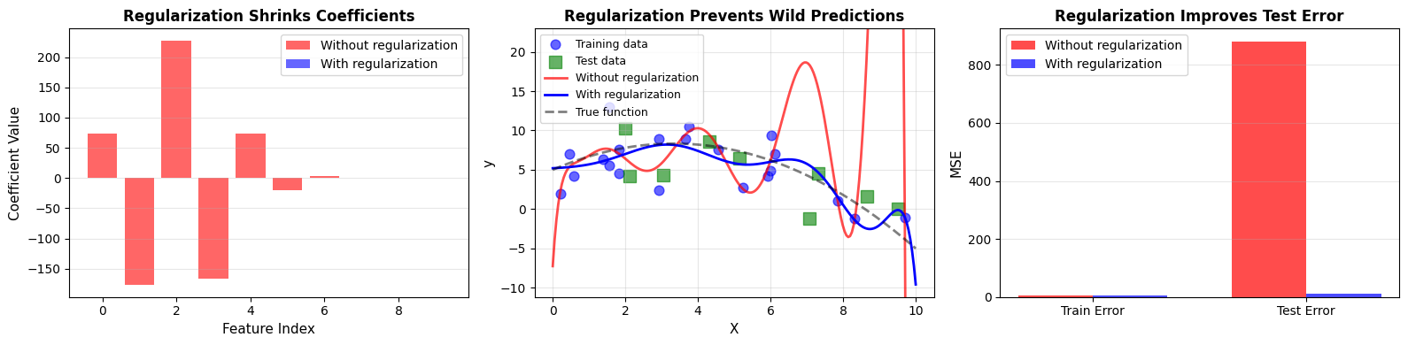
After training both models, we observe a clear pattern:

Without regularization:

• Max coefficient magnitude: 226.94

• Train MSE: 3.84

• Test MSE: 880.95

With regularization:

• Max coefficient magnitude: 0.22

• Train MSE: 6.35

• Test MSE: 11.12

Regularization reduces coefficient magnitudes and improves test performance. The model becomes less extreme, and as a result, more reliable.

---

6.1.7.2. Why Regularization Works

Overfitting arises when a model is too flexible relative to the amount of available data. High flexibility means many parameters. With limited data, those parameters can take extreme values to perfectly match noise.

Regularization counteracts this tendency.

The mechanism is intuitive:

1. Complex models contain many parameters.

2. With limited data, parameters may grow very large to fit small fluctuations.

3. Regularization penalizes large parameter values.

4. The model still captures structure but avoids chasing noise.

The penalty acts as a soft constraint. It does not forbid complexity outright. Instead, it makes complexity costly.

---

6.1.7.3. L2 Regularization (Ridge): Shrinking Weights

Ridge regression introduces an L2 penalty, which is the sum of squared coefficients.

[ \text{Loss}{\text{Ridge}} = \text{MSE} + \alpha \sum{i=1}^{n} w_i^2 ]

Because the penalty squares the coefficients, larger values are penalized more heavily. The effect is smooth shrinkage: coefficients move toward zero but rarely become exactly zero.

Intuition

• Large coefficients become expensive.

• All coefficients shrink proportionally.

• Variance decreases.

• Overfitting is reduced.

The next example demonstrates how increasing α affects both coefficients and error.

from sklearn.linear_model import Ridge

# Generate synthetic data
np.random.seed(42)
n_samples, n_features = 50, 20

X = np.random.randn(n_samples, n_features)
true_coef = np.zeros(n_features)
true_coef[:3] = [5, -3, 2]
y = X @ true_coef + np.random.randn(n_samples) * 2

# Split data
X_train, X_test, y_train, y_test = train_test_split(X, y, test_size=0.3, random_state=42)

alphas = [0, 0.1, 1, 10, 100]
models = {}

Show code cell source

Hide code cell source

# Compare with and without early stopping
# Visualize cross-validation results
# Visualize coefficient differences
# Visualize feature selection
# Compare with and without regularization
fig, axes = plt.subplots(1, 2, figsize=(14, 5))

# Train models with different regularization strengths
for alpha in alphas:
    if alpha == 0:
        model = LinearRegression()
    else:
        model = Ridge(alpha=alpha)

    model.fit(X_train, y_train)
    models[alpha] = model

    axes[0].plot(range(n_features), model.coef_, 'o-', label=f'α={alpha}', alpha=0.7, markersize=6)

axes[0].plot(range(n_features), true_coef, 'k*', markersize=15, label='True coefficients', markeredgewidth=2)
axes[0].axhline(y=0, color='gray', linestyle='--', alpha=0.5)
axes[0].set_xlabel('Feature Index', fontsize=12)
axes[0].set_ylabel('Coefficient Value', fontsize=12)
axes[0].set_title('Ridge: Coefficient Shrinkage', fontsize=13, fontweight='bold')
axes[0].legend(fontsize=9)
axes[0].grid(True, alpha=0.3)

# Calculate errors for different alpha values
train_errors = []
test_errors = []

for alpha in alphas:
    model = models[alpha]
    train_errors.append(mean_squared_error(y_train, model.predict(X_train)))
    test_errors.append(mean_squared_error(y_test, model.predict(X_test)))

axes[1].plot(alphas, train_errors, 'o-', linewidth=2, markersize=8, label='Train MSE')
axes[1].plot(alphas, test_errors, 's-', linewidth=2, markersize=8, label='Test MSE')
axes[1].set_xscale('log')
axes[1].set_xlabel('Regularization Strength (α)', fontsize=12)
axes[1].set_ylabel('MSE', fontsize=12)
axes[1].set_title('Finding Optimal α', fontsize=13, fontweight='bold')
axes[1].legend(fontsize=11)
axes[1].grid(True, alpha=0.3)

plt.tight_layout()
plt.show()

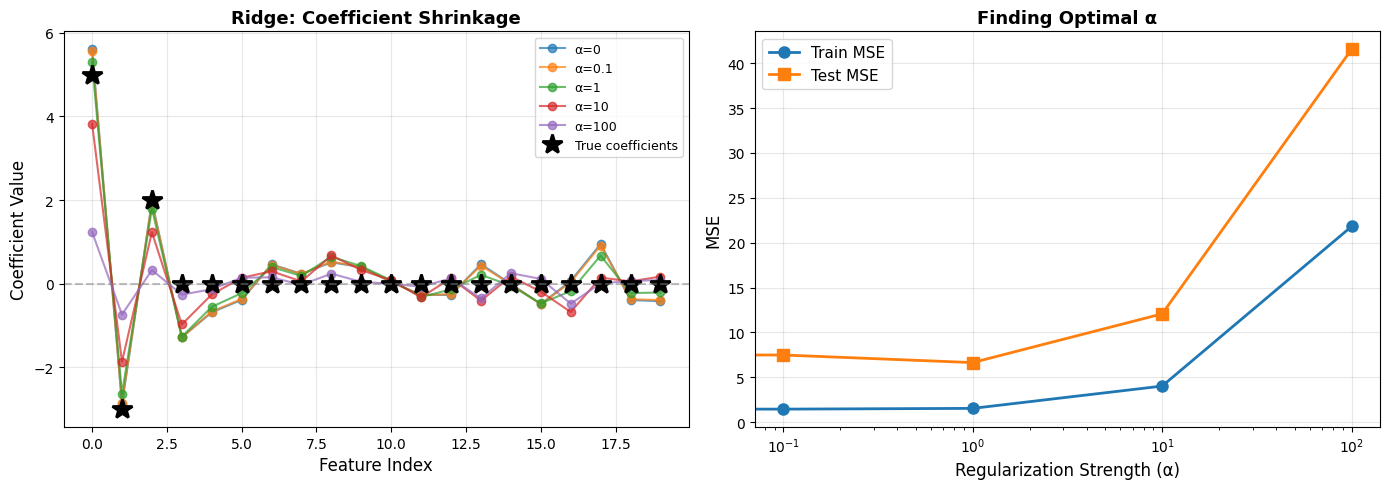
From the experiment:

Key Observations:

1. α = 0 produces large coefficients and overfitting.

2. Small α introduces mild shrinkage.

3. Moderate α achieves the best test performance.

4. Large α forces all coefficients near zero, causing underfitting.

Optimal α for this data: ~1

Ridge regression is particularly useful when features are correlated. Instead of eliminating variables, it distributes weight across them more conservatively.

Tip

Use Ridge (L2) when:

• You have many correlated features

• You want to keep all features but reduce their impact

• You have more features than samples

• Features are on different scales (combine with StandardScaler!)

---

6.1.7.4. L1 Regularization (Lasso): Sparse Solutions

Lasso regression replaces the squared penalty with an absolute value penalty:

[ \text{Loss}{\text{Lasso}} = \text{MSE} + \alpha \sum{i=1}^{n} |w_i| ]

This small mathematical change has a dramatic effect. The L1 penalty encourages exact zeros in the coefficient vector.

Intuition

• Any nonzero coefficient incurs a cost.

• Many coefficients collapse to exactly zero.

• The model performs automatic feature selection.

In contrast to Ridge, which shrinks everything smoothly, Lasso simplifies the model structurally.

Show code cell source

Hide code cell source

from sklearn.linear_model import Lasso

alphas_lasso = [0.01, 0.1, 0.5, 1.0, 5.0]
models_lasso = {}

fig, axes = plt.subplots(1, 2, figsize=(14, 5))

## Train Lasso models with different regularization strengths
for alpha in alphas_lasso:
    model = Lasso(alpha=alpha, max_iter=10000)
    model.fit(X_train, y_train)
    models_lasso[alpha] = model

    axes[0].plot(range(n_features), model.coef_, 'o-', label=f'α={alpha}', alpha=0.7, markersize=6)

axes[0].plot(range(n_features), true_coef, 'k*', markersize=15, label='True coefficients', markeredgewidth=2)
axes[0].axhline(y=0, color='gray', linestyle='--', alpha=0.5)
axes[0].set_xlabel('Feature Index', fontsize=12)
axes[0].set_ylabel('Coefficient Value', fontsize=12)
axes[0].set_title('Lasso: Sparse Solutions', fontsize=13, fontweight='bold')
axes[0].legend(fontsize=9)
axes[0].grid(True, alpha=0.3)

axes[1].bar(range(len(alphas_lasso)),
           [np.sum(models_lasso[alpha].coef_ != 0) for alpha in alphas_lasso],
           color='skyblue', edgecolor='black', linewidth=2)
axes[1].axhline(y=3, color='red', linestyle='--', linewidth=2, label='True number of features')
axes[1].set_xticks(range(len(alphas_lasso)))
axes[1].set_xticklabels([f'{a}' for a in alphas_lasso])
axes[1].set_xlabel('Regularization Strength (α)', fontsize=12)
axes[1].set_ylabel('Number of Non-Zero Coefficients', fontsize=12)
axes[1].set_title('Feature Selection: Lasso Sets Coefficients to Zero', fontsize=13, fontweight='bold')
axes[1].legend()
axes[1].grid(True, alpha=0.3, axis='y')

plt.tight_layout()
plt.show()

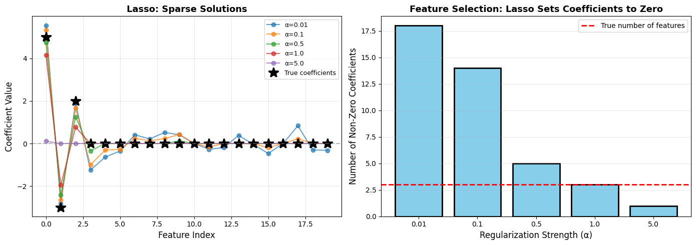
Lasso Feature Selection:

• α=0.01: Selected features: [0, 1, 2, 3, 4, 5, 6, 7, 8, 9, 11, 12, 13, 14, 15, 17, 18, 19], Number: 18/20

• α=0.1: Selected features: [0, 1, 2, 3, 4, 5, 6, 7, 8, 9, 11, 14, 15, 17], Number: 14/20

• α=0.5: Selected features: [0, 1, 2, 3, 9], Number: 5/20 ✓ Correctly identified first 3 features!

• α=1.0: Selected features: [0, 1, 2], Number: 3/20

• α=5.0: Selected features: [0], Number: 1/20

Lasso is especially attractive when interpretability matters. A sparse model is easier to understand and communicate.

---

6.1.7.5. Ridge vs Lasso

When comparing Ridge and Lasso directly, their philosophical difference becomes clear.

Show code cell source

Hide code cell source

alpha_compare = 1.0

fig, axes = plt.subplots(2, 2, figsize=(14, 8))

## Train Ridge and Lasso for comparison
ridge = Ridge(alpha=alpha_compare)
ridge.fit(X_train, y_train)

lasso = Lasso(alpha=alpha_compare, max_iter=10000)
lasso.fit(X_train, y_train)

axes[0, 0].stem(range(n_features), ridge.coef_, linefmt='b-', markerfmt='bo', label='Ridge', basefmt=' ')
axes[0, 0].plot(range(n_features), true_coef, 'k*', markersize=12, label='True')
axes[0, 0].axhline(y=0, color='gray', linestyle='--', alpha=0.5)
axes[0, 0].set_xlabel('Feature Index', fontsize=11)
axes[0, 0].set_ylabel('Coefficient', fontsize=11)
axes[0, 0].set_title(f'Ridge (α={alpha_compare}): All Non-Zero', fontsize=12, fontweight='bold')
axes[0, 0].legend()
axes[0, 0].grid(True, alpha=0.3, axis='y')

axes[0, 1].stem(range(n_features), lasso.coef_, linefmt='r-', markerfmt='ro', label='Lasso', basefmt=' ')
axes[0, 1].plot(range(n_features), true_coef, 'k*', markersize=12, label='True')
axes[0, 1].axhline(y=0, color='gray', linestyle='--', alpha=0.5)
axes[0, 1].set_xlabel('Feature Index', fontsize=11)
axes[0, 1].set_ylabel('Coefficient', fontsize=11)
axes[0, 1].set_title(f'Lasso (α={alpha_compare}): Sparse', fontsize=12, fontweight='bold')
axes[0, 1].legend()
axes[0, 1].grid(True, alpha=0.3, axis='y')

coef_mag_ridge = np.abs(ridge.coef_)
coef_mag_lasso = np.abs(lasso.coef_)

axes[1, 0].bar(range(n_features), coef_mag_ridge, color='blue', alpha=0.6, label='Ridge')
axes[1, 0].set_xlabel('Feature Index', fontsize=11)
axes[1, 0].set_ylabel('|Coefficient|', fontsize=11)
axes[1, 0].set_title('Ridge: Small But Non-Zero', fontsize=12, fontweight='bold')
axes[1, 0].grid(True, alpha=0.3, axis='y')

axes[1, 1].bar(range(n_features), coef_mag_lasso, color='red', alpha=0.6, label='Lasso')
axes[1, 1].set_xlabel('Feature Index', fontsize=11)
axes[1, 1].set_ylabel('|Coefficient|', fontsize=11)
axes[1, 1].set_title('Lasso: Many Exactly Zero', fontsize=12, fontweight='bold')
axes[1, 1].grid(True, alpha=0.3, axis='y')

plt.tight_layout()
plt.show()

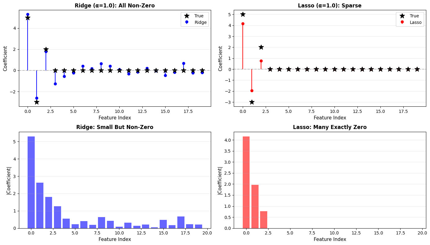
Ridge vs Lasso:

Ridge (L2):

• Non-zero coefficients: 20/20

• Max coefficient: 5.296

• Test MSE: 6.634

Lasso (L1):

• Non-zero coefficients: 3/20

• Max coefficient: 4.161

• Test MSE: 11.113

Aspect	Ridge (L2)	Lasso (L1)
Penalty	Sum of squared coefficients	Sum of absolute coefficients
Effect on coefficients	Shrinks all toward zero	Sets many to exactly zero
Feature selection	No	Yes (automatic)
When to use	Many correlated features	Suspect many features irrelevant
Interpretability	All features contribute	Sparse, easy to interpret
Computational	Has closed-form solution	Requires iterative optimization

Ridge preserves all features with reduced magnitude. Lasso removes many features entirely.

The choice depends on whether you value stability across correlated features or sparsity and interpretability.

6.1.7.6. Elastic Net: Best of Both Worlds

Elastic Net combines both penalties:

[ \text{Loss}_{\text{ElasticNet}} = \text{MSE} + \alpha \rho \sum |w_i| + \alpha (1-\rho) \sum w_i^2 ]

Here:

• α controls overall regularization strength.

• ρ controls the balance between L1 and L2.

When ρ = 0, the model behaves like Ridge. When ρ = 1, it behaves like Lasso.

Elastic Net is particularly useful when features are highly correlated and sparsity is still desirable. It tends to be more stable than pure Lasso while still producing simpler models.

Show code cell source

Hide code cell source

fig, axes = plt.subplots(1, 3, figsize=(16, 4))

## Train Ridge, Lasso, and Elastic Net for comparison
ridge_comp = Ridge(alpha=1.0)
ridge_comp.fit(X_train, y_train)

lasso_comp = Lasso(alpha=0.5, max_iter=10000)
lasso_comp.fit(X_train, y_train)

elastic = ElasticNet(alpha=0.5, l1_ratio=0.5, max_iter=10000)
elastic.fit(X_train, y_train)

models_comp = [
    (ridge_comp, 'Ridge', 'blue'),
    (lasso_comp, 'Lasso', 'red'),
    (elastic, 'Elastic Net', 'green')
]

for ax, (model, name, color) in zip(axes, models_comp):
    ax.stem(range(n_features), model.coef_, linefmt=f'{color[0]}-',
            markerfmt=f'{color[0]}o', label=name, basefmt=' ')
    ax.plot(range(n_features), true_coef, 'k*', markersize=12, label='True')
    ax.axhline(y=0, color='gray', linestyle='--', alpha=0.5)
    ax.set_xlabel('Feature Index', fontsize=11)
    ax.set_ylabel('Coefficient', fontsize=11)
    ax.set_title(f'{name}\n{np.sum(model.coef_ != 0)} non-zero', fontsize=11, fontweight='bold')
    ax.legend(fontsize=9)
    ax.grid(True, alpha=0.3, axis='y')

plt.tight_layout()
plt.show()

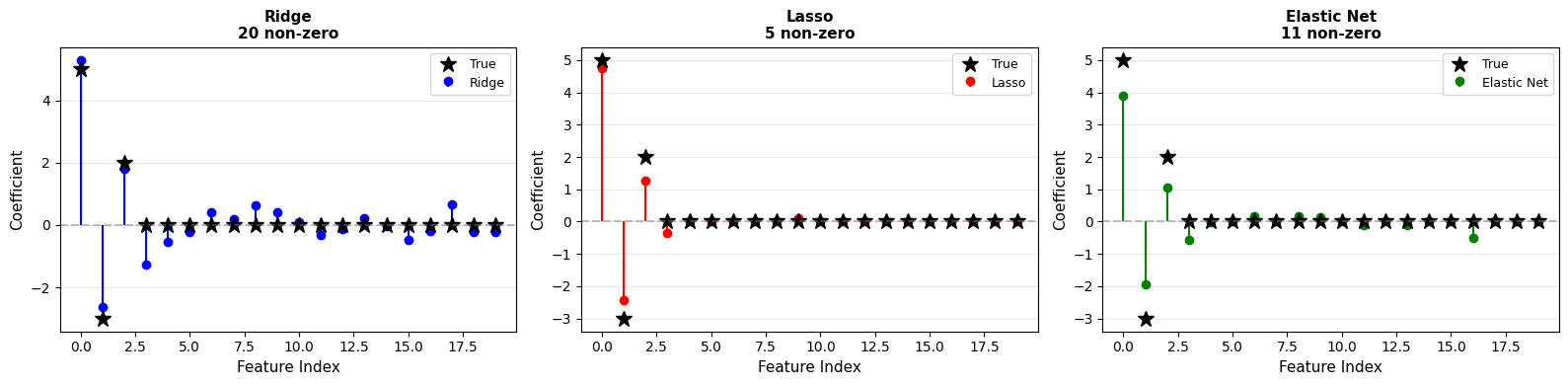
Results:

• Ridge: np.int64(20) non-zero coefficients

• Lasso: np.int64(5) non-zero coefficients

• Elastic Net: np.int64(11) non-zero coefficients

Elastic Net balances sparsity and stability

6.1.7.7. Choosing the Regularization Strength α

The penalty form matters, but the strength of the penalty often matters even more.

• α = 0 means no regularization.

• Small α introduces mild control.

• Large α forces simplicity and risks underfitting.

Selecting α should not rely on guesswork. Cross-validation provides a systematic approach.

How to find the optimal α? Cross-validation!

Show code cell source

Hide code cell source

from sklearn.model_selection import cross_val_score
from sklearn.linear_model import RidgeCV, LassoCV

alphas = np.logspace(-3, 3, 50)

## Find optimal regularization strength via cross-validation
ridge_cv = RidgeCV(alphas=alphas, cv=5)
ridge_cv.fit(X_train, y_train)

lasso_cv = LassoCV(alphas=alphas, cv=5, max_iter=10000)
lasso_cv.fit(X_train, y_train)

LassoCV(alphas=array([1.00000000e-03, 1.32571137e-03, 1.75751062e-03, 2.32995181e-03,
       3.08884360e-03, 4.09491506e-03, 5.42867544e-03, 7.19685673e-03,
       9.54095476e-03, 1.26485522e-02, 1.67683294e-02, 2.22299648e-02,
       2.94705170e-02, 3.90693994e-02, 5.17947468e-02, 6.86648845e-02,
       9.10298178e-02, 1.20679264e-01, 1.59985872e-01, 2.12095089e-01,
       2.81176870e-01, 3.72759372e-0...
       2.68269580e+00, 3.55648031e+00, 4.71486636e+00, 6.25055193e+00,
       8.28642773e+00, 1.09854114e+01, 1.45634848e+01, 1.93069773e+01,
       2.55954792e+01, 3.39322177e+01, 4.49843267e+01, 5.96362332e+01,
       7.90604321e+01, 1.04811313e+02, 1.38949549e+02, 1.84206997e+02,
       2.44205309e+02, 3.23745754e+02, 4.29193426e+02, 5.68986603e+02,
       7.54312006e+02, 1.00000000e+03]),
        cv=5, max_iter=10000)

In a Jupyter environment, please rerun this cell to show the HTML representation or trust the notebook.
On GitHub, the HTML representation is unable to render, please try loading this page with nbviewer.org.

Finding Optimal Regularization Strength

• Ridge best α: 2.6827

• Lasso best α: 0.2812

Show code cell source

Hide code cell source

fig, axes = plt.subplots(1, 2, figsize=(14, 5))

## Ridge CV curve
ridge_scores = []
for alpha in alphas:
    model = Ridge(alpha=alpha)
    scores = cross_val_score(model, X_train, y_train, cv=5, scoring='neg_mean_squared_error')
    ridge_scores.append(-scores.mean())

axes[0].plot(alphas, ridge_scores, 'b-', linewidth=2)
axes[0].axvline(ridge_cv.alpha_, color='red', linestyle='--', linewidth=2, label=f'Best α={ridge_cv.alpha_:.3f}')
axes[0].set_xscale('log')
axes[0].set_xlabel('Regularization Strength (α)', fontsize=12)
axes[0].set_ylabel('Cross-Validation MSE', fontsize=12)
axes[0].set_title('Ridge: Finding Optimal α', fontsize=13, fontweight='bold')
axes[0].legend()
axes[0].grid(True, alpha=0.3)
## Lasso CV curve

lasso_scores = []
for alpha in alphas:
    model = Lasso(alpha=alpha, max_iter=10000)
    scores = cross_val_score(model, X_train, y_train, cv=5, scoring='neg_mean_squared_error')
    lasso_scores.append(-scores.mean())

axes[1].plot(alphas, lasso_scores, 'r-', linewidth=2)
axes[1].axvline(lasso_cv.alpha_, color='blue', linestyle='--', linewidth=2, label=f'Best α={lasso_cv.alpha_:.3f}')
axes[1].set_xscale('log')
axes[1].set_xlabel('Regularization Strength (α)', fontsize=12)
axes[1].set_ylabel('Cross-Validation MSE', fontsize=12)
axes[1].set_title('Lasso: Finding Optimal α', fontsize=13, fontweight='bold')
axes[1].legend()
axes[1].grid(True, alpha=0.3)

plt.tight_layout()
plt.show()

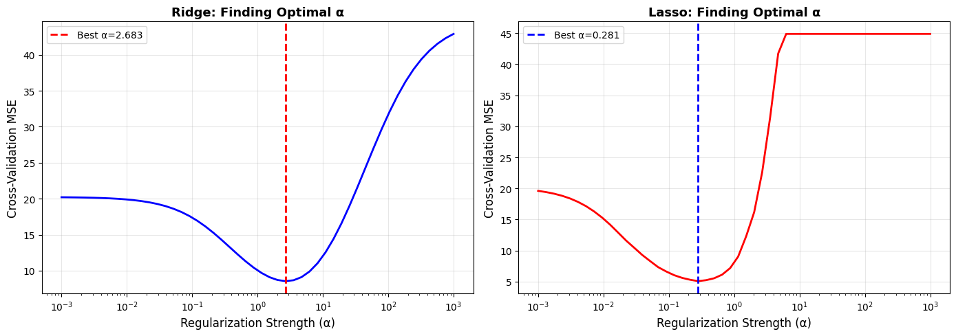
Cross-validation curves make the tradeoff visible: too little regularization increases variance, too much increases bias. The minimum point balances both.

Optimal models found via cross-validation:

• Ridge test MSE: 6.989

• Lasso test MSE: 5.981

Tip

Best Practice for Choosing α:

1. Start with a wide logarithmic range.

2. Use cross-validation tools such as RidgeCV or LassoCV.

3. For Elastic Net, tune both α and l1_ratio.

4. Visualize the validation curve.

5. Evaluate the final choice on a held-out test set.

6.1.7.8. Beyond Linear Models

Regularization is not limited to linear regression. The principle of controlling complexity appears across machine learning.

Dropout

In neural networks, dropout randomly disables neurons during training. This prevents units from becoming overly dependent on one another and improves generalization.

Dropout: Randomly “drop” (set to zero) neurons during training

Effect: Prevents co-adaptation of neurons, reduces overfitting

## Conceptual example (PyTorch style)
import torch.nn as nn

model = nn.Sequential(
    nn.Linear(100, 50),
    nn.ReLU(),
    nn.Dropout(p=0.5),  ## Drop 50% of neurons
    nn.Linear(50, 10)
)

Early Stopping

Another form of regularization does not modify the objective function at all. Instead, it limits training duration.

As training proceeds, training error often decreases steadily. Validation error, however, eventually begins to increase. Stopping at the minimum validation error prevents the model from overfitting.

Early Stopping: Stop training when validation error stops improving

Effect: Prevents model from overfitting by not training too long

Show code cell source

Hide code cell source

np.random.seed(42)

epochs = 100
train_errors = []
val_errors = []

for epoch in range(epochs):
    train_err = 10 * np.exp(-epoch/20) + 0.5

    if epoch < 30:
        val_err = 10 * np.exp(-epoch/15) + 1.0
    else:
        val_err = 10 * np.exp(-30/15) + 1.0 + 0.05 * (epoch - 30)

    train_errors.append(train_err)
    val_errors.append(val_err)

best_epoch = np.argmin(val_errors)

plt.figure(figsize=(10, 6))
plt.plot(train_errors, 'b-', linewidth=2, label='Training Error')
plt.plot(val_errors, 'r-', linewidth=2, label='Validation Error')
plt.axvline(best_epoch, color='green', linestyle='--', linewidth=2,
           label=f'Early Stop (epoch {best_epoch})')
plt.scatter([best_epoch], [val_errors[best_epoch]], s=200, c='green',
           marker='*', edgecolors='black', linewidths=2, zorder=5)
plt.xlabel('Epoch', fontsize=12)
plt.ylabel('Error', fontsize=12)
plt.title('Early Stopping: Stop When Validation Error Increases', fontsize=14, fontweight='bold')
plt.legend(fontsize=11)
plt.grid(True, alpha=0.3)
plt.tight_layout()
plt.show()

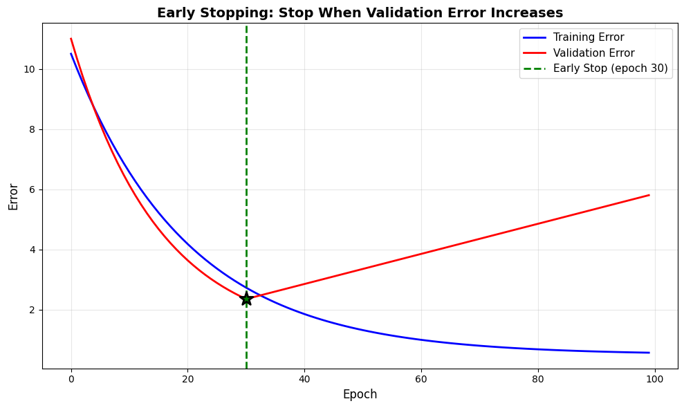
Early Stopping:

• Best validation error at epoch: np.int64(30)

• If we continued to epoch 100:

  • Training error would be: 0.57 (keeps improving)

  • Validation error would be: 5.80 (gets worse!)

  • Early stopping prevents overfitting without modifying the model

Data Augmentation

Data augmentation increases the effective size of the dataset by generating new examples from existing ones. By exposing the model to more variation, it reduces overfitting without changing the model structure.

Examples include:

• Image transformations such as rotation and flipping

• Text transformations such as synonym replacement

• Time series perturbations such as noise injection

Effect: Increases effective dataset size, reduces overfitting

Examples:

• Images: Rotate, flip, crop, color jitter

• Text: Synonym replacement, back-translation

• Time series: Time warping, noise injection

6.1.7.9. Practical Guidelines

Note

When to Use Which Regularization:

Use Ridge (L2) when:

• All features may be relevant

• Features are correlated

• Smooth shrinkage is desired

Use Lasso (L1) when:

• Many features are likely irrelevant

• Interpretability is important

• Automatic feature selection is needed

Use Elastic Net when:

• You want both stability and sparsity

• Correlated feature groups exist

• Features outnumber samples

Use Dropout when:

• Training deep neural networks

Use Early Stopping when:

• Training iterative models

• Validation error begins to increase

• Computational resources are limited