6.2.3.4. Deep Learning and Practical Tips#
The Neural Networks chapter showed that stacking layers dramatically improves performance. But going deep - 5, 10, 50 layers - introduces new problems that must be solved for training to succeed at all. This chapter covers those problems and the solutions that made the modern deep learning revolution possible.
It closes with a complete practical workflow for training, debugging, and regularising a network using scikit-learn’s MLPClassifier.
Scope note: Deep learning is an enormous field. This chapter focuses on fully-connected feedforward networks. Specialised architectures - CNNs (images), RNNs / LSTMs (sequences), Transformers (language) - build directly on these foundations but are outside the scope of this introduction.
The Core Idea: Depth Enables Hierarchy#
Deeper networks learn hierarchical representations: early layers detect simple local patterns; later layers compose them into complex abstractions. This is more parameter-efficient than making a single very wide layer.
However, training a deep network means gradients must flow backwards through many layers, and two failure modes emerge:
Vanishing gradients - gradients shrink exponentially toward the first layer; early layers stop learning.
Exploding gradients - gradients grow exponentially; training diverges.
The Math: Why Gradients Vanish#
Backpropagation multiplies gradient terms layer by layer via the chain rule:
Each term \(\frac{\partial \mathbf{a}^{(\ell)}}{\partial \mathbf{a}^{(\ell-1)}} = W^{(\ell)} \odot f'(\mathbf{z}^{(\ell)})\) involves the derivative of the activation function. For sigmoid and tanh, this derivative is \(\leq 0.25\) or \(\leq 1\) respectively, and saturates near zero for large activations. Multiplying \(L\) such small numbers together gives an exponentially tiny gradient.
ReLU solves this: \(f'(z) = 1\) for \(z > 0\), so gradients are passed through undiminished for active neurons.
Solutions to Training Deep Networks#
1. Use ReLU (and Variants)#
ReLU eliminates gradient saturation for positive activations. Variants handle the “dead neuron” problem (ReLU outputs exactly 0 for \(z < 0\), permanently killing gradient flow):
Activation |
Formula |
Notes |
|---|---|---|
ReLU |
\(\max(0, z)\) |
Fast, default choice |
Leaky ReLU |
\(\max(0.01z, z)\) |
Small gradient for \(z < 0\) |
ELU |
\(z\) if \(z>0\), else \(\alpha(e^z-1)\) |
Smooth, negative outputs |
2. Batch Normalisation#
Normalises the activations within each mini-batch to have zero mean and unit variance, then rescales with learned parameters \(\gamma\) and \(\beta\):
Benefits: faster convergence, less sensitivity to weight initialisation, mild regularisation effect.
3. Dropout#
During each training step, randomly zero out a fraction \(p\) of neurons. This forces the network to learn redundant representations - it can no longer rely on any one neuron always being present:
At test time, all neurons are active but their outputs are scaled by \((1-p)\) to maintain the same expected activation. Typical values: \(p = 0.2\)–\(0.5\).
4. Weight Initialisation#
Uninitialised or poorly-initialised weights lead to vanishing or exploding activations from the first forward pass. He initialisation (for ReLU) scales weights by \(\sqrt{2/n_\text{in}}\):
scikit-learn uses a suitable initialisation automatically.
5. Early Stopping#
Monitor validation loss during training. When it stops improving, halt training and restore the best weights. This prevents overfitting without changing the architecture.
In scikit-learn#
MLPClassifier exposes the key practical knobs:
from sklearn.neural_network import MLPClassifier

mlp = MLPClassifier(
    hidden_layer_sizes=(256, 128, 64),   # 3 hidden layers
    activation='relu',
    solver='adam',
    alpha=1e-3,                           # L2 regularisation (weight decay)
    learning_rate='adaptive',             # halve lr when training loss stops improving
    learning_rate_init=0.001,
    early_stopping=True,                  # hold out 10% of training data for validation
    validation_fraction=0.1,
    n_iter_no_change=15,                  # patience
    max_iter=500,
    random_state=42,
    verbose=False,
)
Note: scikit-learn’s MLP does not support batch normalisation or dropout directly. For those, use PyTorch or Keras/TensorFlow - the standard frameworks for production deep learning. scikit-learn’s MLP is ideal for tabular data with up to a few hundred thousand samples.
Example: Complete Training Workflow#
from sklearn.neural_network import MLPClassifier

mlp = MLPClassifier(
    hidden_layer_sizes=(256, 128, 64),
    activation='relu',
    solver='adam',
    alpha=1e-3,
    learning_rate='adaptive',
    learning_rate_init=0.001,
    early_stopping=True,
    validation_fraction=0.1,
    n_iter_no_change=20,
    max_iter=500,
    random_state=42,
)
mlp.fit(X_train_sc, y_train)

train_acc = accuracy_score(y_train, mlp.predict(X_train_sc))
test_acc  = accuracy_score(y_test,  mlp.predict(X_test_sc))
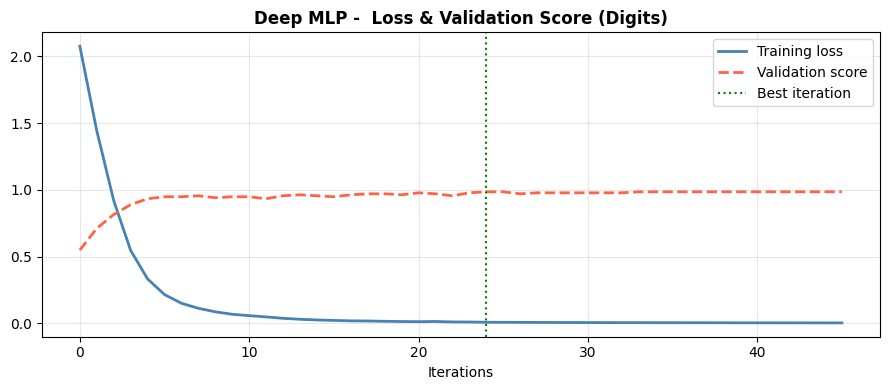
The three-layer network with early stopping achieves 0.978 test accuracy. The adaptive learning rate and early stopping cooperate: the learning rate decreases when the training loss plateaus, and training halts before the validation score degrades.
Training and Validation Loss#
fig, ax = plt.subplots(figsize=(9, 4))
ax.plot(mlp.loss_curve_,         label='Training loss',   color='steelblue', lw=2)
ax.plot(mlp.validation_scores_,  label='Validation score', color='tomato',   lw=2, ls='--')
ax.axvline(np.argmax(mlp.validation_scores_), color='green', lw=1.5, ls=':', label='Best iteration')
ax.set_xlabel("Iterations")
ax.set_title("Deep MLP -  Loss & Validation Score (Digits)", fontweight='bold')
ax.legend()
ax.grid(True, alpha=0.3)
plt.tight_layout()
plt.show()
Classification Report#
print(classification_report(y_test, mlp.predict(X_test_sc), target_names=[str(d) for d in range(10)]))
              precision    recall  f1-score   support

           0       1.00      0.98      0.99        45
           1       0.94      0.96      0.95        46
           2       0.96      1.00      0.98        44
           3       1.00      1.00      1.00        46
           4       0.98      1.00      0.99        45
           5       1.00      0.98      0.99        46
           6       1.00      1.00      1.00        45
           7       0.96      1.00      0.98        45
           8       1.00      0.86      0.93        43
           9       0.96      1.00      0.98        45

    accuracy                           0.98       450
   macro avg       0.98      0.98      0.98       450
weighted avg       0.98      0.98      0.98       450
Regularisation: Effect of Alpha#
The alpha parameter controls L2 weight decay - how strongly large weights are penalised. Higher alpha → smoother, more regularised model.
alphas    = [1e-5, 1e-4, 1e-3, 1e-2, 1e-1, 1.0]
train_acc_list, test_acc_list = [], []

for a in alphas:
    m = MLPClassifier(hidden_layer_sizes=(256, 128, 64), activation='relu',
                      solver='adam', alpha=a, max_iter=400, random_state=42)
    m.fit(X_train_sc, y_train)
    train_acc_list.append(accuracy_score(y_train, m.predict(X_train_sc)))
    test_acc_list.append(accuracy_score(y_test,   m.predict(X_test_sc)))

fig, ax = plt.subplots(figsize=(9, 4))
ax.semilogx(alphas, train_acc_list, 'o-', label='Train Accuracy', color='steelblue')
ax.semilogx(alphas, test_acc_list,  's-', label='Test Accuracy',  color='tomato')
ax.set_xlabel("alpha (L2 regularisation)")
ax.set_ylabel("Accuracy")
ax.set_title("Effect of L2 Regularisation (alpha) -  Deep MLP", fontweight='bold')
ax.legend()
ax.grid(True, alpha=0.3)
plt.tight_layout()
plt.show()
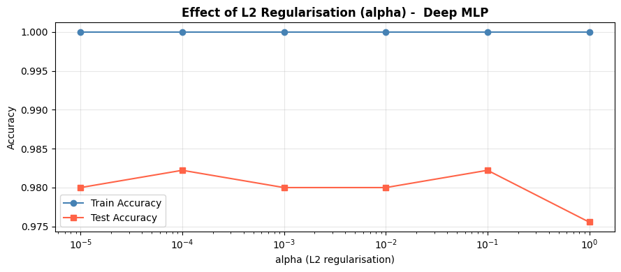
Very low alpha: the model overfits (train ≫ test). Very high alpha: the model is too constrained (both low). The optimal alpha sits in the flat region where test accuracy is maximised.