6.3.1.4. Cluster Evaluation: Measuring Quality

You have learned how to perform clustering using K-Means Clustering, Hierarchical Clustering, and DBSCAN: Density-Based Clustering methods. The natural next question is: how do we know whether the clusters we obtained are actually good?

Unlike supervised learning, clustering does not usually come with ground truth labels. There is no direct accuracy measure. Instead, we must evaluate clusters indirectly by measuring their internal structure.

A good clustering should satisfy two key properties:

1. Cohesion: Points within the same cluster should be similar to one another.

2. Separation: Points in different clusters should be clearly distinct.

Cluster evaluation metrics are designed to quantify these ideas.

---

The Challenge: No Ground Truth

In supervised learning, we compare predictions against known labels. In clustering, we typically have no such labels. This makes evaluation inherently more subtle.

There are two broad categories of evaluation metrics:

1. Internal Metrics

These rely only on the feature data (X). They assess how well the clustering structure fits the data itself.

• Silhouette Score

• Davies-Bouldin Index

• Calinski-Harabasz Index

2. External Metrics

These require true labels. They are used when ground truth is available for validation purposes.

• Adjusted Rand Index (ARI)

• Normalized Mutual Information (NMI)

In most real applications, internal metrics are the primary tools, since labels are rarely available.

Show code cell source

Hide code cell source

import numpy as np
import pandas as pd
import matplotlib.pyplot as plt
from myst_nb import glue
from sklearn.cluster import KMeans, DBSCAN, AgglomerativeClustering
from sklearn.datasets import make_blobs, load_iris
from sklearn.metrics import (silhouette_score, silhouette_samples,
                             davies_bouldin_score, calinski_harabasz_score,
                             adjusted_rand_score, normalized_mutual_info_score)
from sklearn.preprocessing import StandardScaler

np.random.seed(42)

X_sil, y_true = make_blobs(n_samples=300, centers=3,
                            cluster_std=0.7, random_state=42)

Silhouette Score: The Most Widely Used Metric

The Silhouette Score evaluates how well each point fits within its assigned cluster compared to other clusters.

For each point (i):

• a(i): Average distance to other points in the same cluster

• b(i): Average distance to points in the nearest neighboring cluster

• s(i) = \(\frac{b(i) - a(i)}{\max(a(i), b(i))}\)

Interpretation of (s(i)):

• +1: The point is well matched to its own cluster and far from others

• 0: The point lies near a cluster boundary

• -1: The point may be assigned to the wrong cluster

The overall Silhouette Score is simply the average of (s(i)) across all data points.

The following experiment compares silhouette scores for different values of (k).

# Try different k values
k_values = [2, 3, 4, 5]

fig, axes = plt.subplots(2, 2, figsize=(14, 12))
axes = axes.ravel()

for idx, k in enumerate(k_values):
    kmeans = KMeans(n_clusters=k, init='k-means++', n_init=10, random_state=42)
    labels = kmeans.fit_predict(X_sil)

    # Compute silhouette
    sil_score = silhouette_score(X_sil, labels)
    sil_samples = silhouette_samples(X_sil, labels)

    # Plot clusters
    colors = ['red', 'blue', 'green', 'orange', 'purple']
    for cluster_id in range(k):
        cluster_mask = labels == cluster_id
        axes[idx].scatter(X_sil[cluster_mask, 0], X_sil[cluster_mask, 1],
                         s=60, c=colors[cluster_id], alpha=0.6,
                         edgecolors='black', linewidths=0.5,
                         label=f'C{cluster_id} (sil={sil_samples[cluster_mask].mean():.2f})')

    axes[idx].scatter(kmeans.cluster_centers_[:, 0],
                     kmeans.cluster_centers_[:, 1],
                     s=300, c='yellow', marker='*',
                     edgecolors='black', linewidths=2)

    axes[idx].set_xlabel('Feature 1', fontsize=11)
    axes[idx].set_ylabel('Feature 2', fontsize=11)
    axes[idx].set_title(f'k={k}\nSilhouette Score: {sil_score:.3f}',
                       fontsize=12, fontweight='bold')
    axes[idx].legend(loc='best', fontsize=8)
    axes[idx].grid(True, alpha=0.3)

plt.tight_layout()
plt.show()

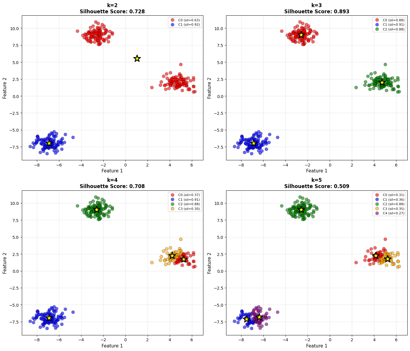
As you examine the plots, notice how both cluster structure and silhouette score change with (k). The optimal number of clusters typically corresponds to a high average silhouette value and visually well-separated groups.

Davies-Bouldin Index: Measuring Cluster Similarity

The Davies-Bouldin Index quantifies how similar each cluster is to its most similar neighboring cluster.

• It compares within-cluster scatter to between-cluster separation.

• It penalizes clusters that overlap or are poorly separated.

• Lower values indicate better clustering.

• A value close to 0 represents strong separation.

Unlike the silhouette score, which is bounded between -1 and 1, the Davies-Bouldin Index has no fixed upper bound. Interpretation relies on relative comparison across models.

# Compare different k values
k_range = range(2, 8)
db_scores = []
sil_scores = []

for k in k_range:
    kmeans = KMeans(n_clusters=k, init='k-means++', n_init=10, random_state=42)
    labels = kmeans.fit_predict(X_sil)

    db_score = davies_bouldin_score(X_sil, labels)
    sil_score = silhouette_score(X_sil, labels)

    db_scores.append(db_score)
    sil_scores.append(sil_score)

# Plot
fig, axes = plt.subplots(1, 2, figsize=(14, 5))

# Davies-Bouldin (lower better)
axes[0].plot(k_range, db_scores, 'o-', linewidth=2, markersize=8, color='red')
axes[0].axvline(x=3, color='green', linestyle='--', linewidth=2,
               label='True k=3')
axes[0].set_xlabel('Number of Clusters (k)', fontsize=12)
axes[0].set_ylabel('Davies-Bouldin Index', fontsize=12)
axes[0].set_title('Davies-Bouldin Index\n(Lower is Better)',
                  fontsize=13, fontweight='bold')
axes[0].legend()
axes[0].grid(True, alpha=0.3)

# Silhouette (higher better)
axes[1].plot(k_range, sil_scores, 'o-', linewidth=2, markersize=8, color='blue')
axes[1].axvline(x=3, color='green', linestyle='--', linewidth=2,
               label='True k=3')
axes[1].set_xlabel('Number of Clusters (k)', fontsize=12)
axes[1].set_ylabel('Silhouette Score', fontsize=12)
axes[1].set_title('Silhouette Score\n(Higher is Better)',
                  fontsize=13, fontweight='bold')
axes[1].legend()
axes[1].grid(True, alpha=0.3)

plt.tight_layout()
plt.show()

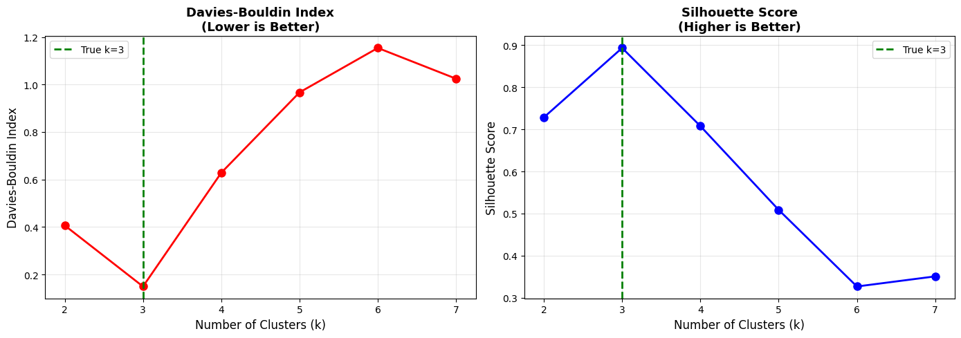
When comparing different values of (k), look for the configuration that minimizes the Davies-Bouldin score while maintaining interpretability.

Calinski-Harabasz Index: The Variance Ratio

The Calinski-Harabasz Index, also known as the Variance Ratio Criterion, evaluates the ratio of:

• Between-cluster dispersion

• Within-cluster dispersion

Intuitively, good clustering should maximize separation between clusters while minimizing variation inside clusters.

• Higher values indicate better-defined clusters.

# Compute for different k
ch_scores = []

for k in k_range:
    kmeans = KMeans(n_clusters=k, init='k-means++', n_init=10, random_state=42)
    labels = kmeans.fit_predict(X_sil)
    ch_score = calinski_harabasz_score(X_sil, labels)
    ch_scores.append(ch_score)

# Plot all three metrics together
fig, axes = plt.subplots(1, 3, figsize=(16, 5))

# Silhouette
axes[0].plot(k_range, sil_scores, 'o-', linewidth=2, markersize=8, color='blue')
axes[0].axvline(x=3, color='red', linestyle='--', linewidth=2, label='Best k')
axes[0].set_xlabel('k', fontsize=12)
axes[0].set_ylabel('Silhouette Score', fontsize=12)
axes[0].set_title('Silhouette\n(Higher Better)', fontsize=12, fontweight='bold')
axes[0].legend()
axes[0].grid(True, alpha=0.3)

# Davies-Bouldin
axes[1].plot(k_range, db_scores, 'o-', linewidth=2, markersize=8, color='red')
axes[1].axvline(x=3, color='green', linestyle='--', linewidth=2, label='Best k')
axes[1].set_xlabel('k', fontsize=12)
axes[1].set_ylabel('Davies-Bouldin Index', fontsize=12)
axes[1].set_title('Davies-Bouldin\n(Lower Better)', fontsize=12, fontweight='bold')
axes[1].legend()
axes[1].grid(True, alpha=0.3)

# Calinski-Harabasz
axes[2].plot(k_range, ch_scores, 'o-', linewidth=2, markersize=8, color='green')
axes[2].axvline(x=3, color='red', linestyle='--', linewidth=2, label='Best k')
axes[2].set_xlabel('k', fontsize=12)
axes[2].set_ylabel('Calinski-Harabasz Score', fontsize=12)
axes[2].set_title('Calinski-Harabasz\n(Higher Better)', fontsize=12, fontweight='bold')
axes[2].legend()
axes[2].grid(True, alpha=0.3)

plt.tight_layout()
plt.show()

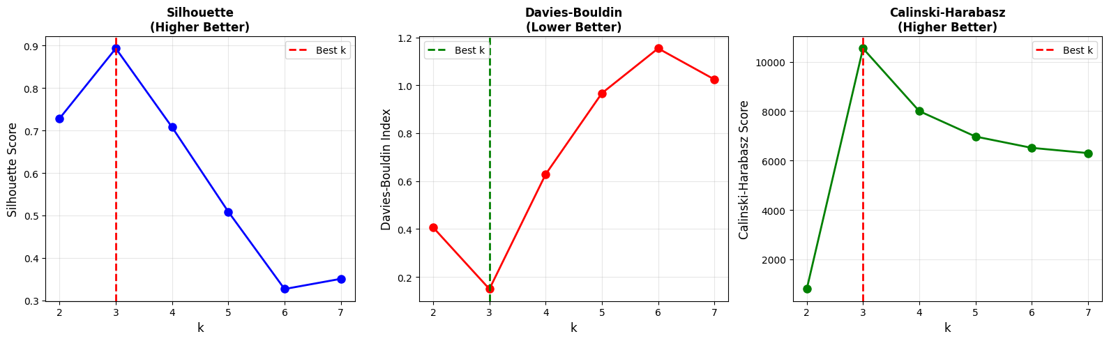
When multiple metrics agree on the same value of (k), confidence in that clustering choice increases.

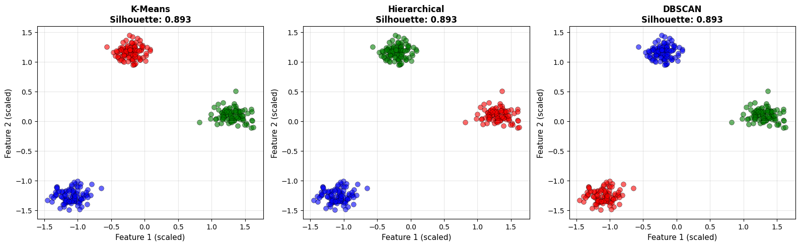
Comparing Algorithms

Evaluation metrics are also useful for comparing different clustering algorithms on the same dataset.

Here we compare:

• K-Means

• Hierarchical Clustering

• DBSCAN

All models are applied to standardized data to ensure fair comparison. Distance-based metrics are highly sensitive to feature scale, so standardization is essential.

# Scale data
scaler = StandardScaler()
X_sil_scaled = scaler.fit_transform(X_sil)

# Try different algorithms
algorithms = {
    'K-Means': KMeans(n_clusters=3, init='k-means++', n_init=10, random_state=42),
    'Hierarchical': AgglomerativeClustering(n_clusters=3, linkage='ward'),
    'DBSCAN': DBSCAN(eps=0.5, min_samples=5)
}

results = []

fig, axes = plt.subplots(1, 3, figsize=(16, 5))

for idx, (name, algo) in enumerate(algorithms.items()):
    labels = algo.fit_predict(X_sil_scaled)

    # Skip DBSCAN if only noise
    n_clusters = len(set(labels)) - (1 if -1 in labels else 0)

    if n_clusters > 1:
        sil = silhouette_score(X_sil_scaled, labels)
        db = davies_bouldin_score(X_sil_scaled, labels)
        ch = calinski_harabasz_score(X_sil_scaled, labels)
    else:
        sil, db, ch = np.nan, np.nan, np.nan

    results.append({
        'Algorithm': name,
        'Clusters': n_clusters,
        'Silhouette': sil,
        'Davies-Bouldin': db,
        'Calinski-Harabasz': ch
    })

    # Plot
    unique_labels = set(labels)
    colors = ['red', 'blue', 'green', 'orange']

    for k in unique_labels:
        if k == -1:  # Noise
            class_mask = labels == k
            axes[idx].scatter(X_sil_scaled[class_mask, 0],
                            X_sil_scaled[class_mask, 1],
                            s=50, c='gray', marker='x', alpha=0.5)
        else:
            class_mask = labels == k
            axes[idx].scatter(X_sil_scaled[class_mask, 0],
                            X_sil_scaled[class_mask, 1],
                            s=50, c=colors[k % len(colors)], alpha=0.6,
                            edgecolors='black', linewidths=0.5)

    axes[idx].set_xlabel('Feature 1 (scaled)', fontsize=11)
    axes[idx].set_ylabel('Feature 2 (scaled)', fontsize=11)
    if not np.isnan(sil):
        axes[idx].set_title(f'{name}\nSilhouette: {sil:.3f}',
                           fontsize=12, fontweight='bold')
    else:
        axes[idx].set_title(f'{name}\n(Evaluation failed)',
                           fontsize=12, fontweight='bold')
    axes[idx].grid(True, alpha=0.3)

plt.tight_layout()
plt.show()

results_df = pd.DataFrame(results)
display(results_df)

	Algorithm	Clusters	Silhouette	Davies-Bouldin	Calinski-Harabasz
0	K-Means	3	0.893395	0.148312	9577.258358
1	Hierarchical	3	0.893395	0.148312	9577.258358
2	DBSCAN	3	0.893395	0.148312	9577.258358

Notice that different algorithms may produce different numbers of clusters. Metrics help quantify quality, but visualization remains critical. A strong metric score does not automatically imply meaningful structure.

External Metrics: When Labels Are Available

Occasionally, you may have ground truth labels available for validation. In such cases, external metrics provide a direct way to measure agreement between predicted clusters and true classes.

Two common external metrics:

• Adjusted Rand Index (ARI)

  • Range: [-1, 1]

  • 1 indicates perfect agreement

• Normalized Mutual Information (NMI)

  • Range: [0, 1]

  • 1 indicates perfect agreement

Unlike internal metrics, external metrics evaluate alignment with known labels rather than structural properties alone.

Show code cell source

Hide code cell source

# Use Iris with known species labels
iris = load_iris()
X_iris = iris.data
y_iris = iris.target

X_iris_scaled = scaler.fit_transform(X_iris)

kmeans_iris = KMeans(n_clusters=3, init='k-means++', n_init=10, random_state=42)
labels_pred = kmeans_iris.fit_predict(X_iris_scaled)

ari = adjusted_rand_score(y_iris, labels_pred)
nmi = normalized_mutual_info_score(y_iris, labels_pred)
sil = silhouette_score(X_iris_scaled, labels_pred)
db  = davies_bouldin_score(X_iris_scaled, labels_pred)

glue('iris-ari', round(ari, 3), display=False)
glue('iris-nmi', round(nmi, 3), display=False)
glue('iris-sil', round(sil, 3), display=False)
glue('iris-db',  round(db,  3), display=False)

fig, axes = plt.subplots(1, 2, figsize=(14, 6))

for ax, labels_plot, title in zip(
        axes,
        [y_iris, labels_pred],
        ['True Species (Ground Truth)',
         f'K-Means  |  ARI = {ari:.3f}, NMI = {nmi:.3f}']):
    for cls in np.unique(labels_plot):
        mask = labels_plot == cls
        ax.scatter(X_iris_scaled[mask, 0], X_iris_scaled[mask, 2],
                   s=60, alpha=0.7, edgecolors='black', linewidths=0.5,
                   label=f'Class {cls}')
    ax.set_xlabel('Sepal length (scaled)', fontsize=12)
    ax.set_ylabel('Petal length (scaled)', fontsize=12)
    ax.set_title(title, fontsize=13, fontweight='bold')
    ax.legend(); ax.grid(True, alpha=0.3)

plt.tight_layout()
plt.show()

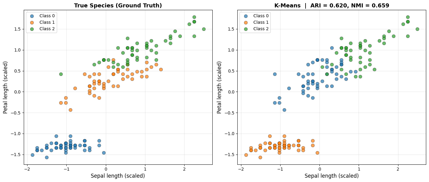
K-Means achieves an ARI of 0.62 and an NMI of 0.659, with an internal silhouette score of 0.46 and a Davies-Bouldin index of 0.834. The high ARI confirms that the discovered clusters closely align with the true species labels.

External metrics are useful for validation, but they should not be used for selecting models in purely unsupervised settings.

Practical Recommendations

Choosing the Number of Clusters

Use the Silhouette Score as your primary indicator. Combine it with the elbow method for K-Means when appropriate. Davies-Bouldin and Calinski-Harabasz provide complementary perspectives.

Look for agreement across multiple metrics rather than relying on a single number.

---

Comparing Algorithms

• Always compute metrics on the same standardized dataset.

• Visualize clusters alongside metrics.

• Be cautious with non-spherical or density-based structures where certain metrics may be misleading.

Metrics quantify structure, but interpretation requires context.

---

Silhouette Score Guidelines

Range	Interpretation
0.70 – 1.00	Strong structure
0.50 – 0.70	Reasonable structure
0.25 – 0.50	Weak structure
< 0.25	No substantial structure

These ranges provide general intuition, not strict rules.

---

Common Pitfalls

• Optimizing a metric too aggressively can produce artificial solutions.

• Failing to standardize features makes distance-based metrics unreliable.

• High metric scores do not guarantee business relevance.

Domain knowledge often overrides small numerical differences. A cluster structure that supports meaningful decisions is more valuable than a marginal improvement in silhouette score.

---

Key Takeaways

Important

Remember These Points:

1. Internal Metrics (No Labels)

   • Silhouette Score: [-1, 1], higher better

   • Davies-Bouldin: [0, ∞), lower better

   • Calinski-Harabasz: [0, ∞), higher better

2. External Metrics (Need Labels)

   • Adjusted Rand Index: [-1, 1], 1 = perfect match

   • Normalized Mutual Info: [0, 1], 1 = perfect match

   • Use for validation, not primary model selection

3. Silhouette Score (Most Used)

   • Measures cohesion and separation

   • Provides per-sample and overall insight

   • Helpful for choosing k

4. Practical Workflow

   • Compute multiple internal metrics

   • Look for agreement across metrics

   • Visualize clusters

   • Apply domain knowledge

   • Iterate

5. Limitations

   • Metrics may disagree

   • No single metric is perfect

   • Visualization remains essential

6. Best Practice

   • Use Silhouette as primary metric

   • Davies-Bouldin as secondary check

   • Always visualize results

   • Validate with domain experts

Cluster evaluation is not about finding a perfect score. It is about combining quantitative metrics, visual inspection, and domain understanding to arrive at meaningful structure in data.