6.2.1.1. Metrics and Loss Functions#
Before training any regression model, we need a way to answer a fundamental question: how good is a prediction? Two numbers are involved - the true value \(y\) and the predicted value \(\hat{y}\) - and we need a single number that captures how far apart they are.
This single number is called a loss (or cost) when used to guide training, and a metric when used to evaluate a trained model. The distinction matters:
Loss functions need to be mathematically convenient for optimisation (e.g. differentiable). The model minimises the loss during training.
Evaluation metrics are chosen to be interpretable and meaningful for the problem at hand. They are computed after training to communicate model quality.
Loss Functions#
Mean Squared Error (MSE)#
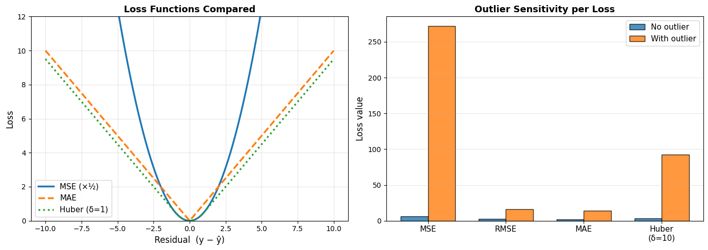
MSE is the workhorse of regression. Squaring the errors has two effects: it makes the result always non-negative, and it penalises large errors disproportionately - a prediction that is 10 units off contributes 100 times as much as one that is 1 unit off. This makes MSE sensitive to outliers.
Properties:
Differentiable everywhere → easy to optimise with gradient descent
Strongly penalises large deviations
Units are squared (e.g. dollars²) - less intuitive
def mse(y_true, y_pred):
    return np.mean((y_true - y_pred) ** 2)

pd.DataFrame({
    "Predictions": ["Good", "Poor", "With one outlier"],
    "MSE": [mse(y_true, y_pred_good), mse(y_true, y_pred_poor), mse(y_true, y_pred_outlier)],
}).round(2)
| Predictions | MSE | |
|---|---|---|
| 0 | Good | 6.04 |
| 1 | Poor | 256.19 |
| 2 | With one outlier | 271.80 |
On the example data, good predictions yield an MSE of 6.04; introducing a single outlier inflates this to 271.8 - a dramatic increase caused by squaring one large residual.
Root Mean Squared Error (RMSE)#
RMSE is simply the square root of MSE, restoring the original units. It is the most commonly reported regression error because it is on the same scale as the target variable and still penalises large errors.
Properties:
Same units as \(y\) → directly interpretable
Still sensitive to outliers (inherits MSE’s squared penalty)
Lower is better; RMSE = 0 means perfect predictions
def rmse(y_true, y_pred):
    return np.sqrt(mse(y_true, y_pred))

pd.DataFrame({
    "Predictions": ["Good", "Poor", "With one outlier"],
    "RMSE": [rmse(y_true, y_pred_good), rmse(y_true, y_pred_poor), rmse(y_true, y_pred_outlier)],
}).round(2)
| Predictions | RMSE | |
|---|---|---|
| 0 | Good | 2.46 |
| 1 | Poor | 16.01 |
| 2 | With one outlier | 16.49 |
Good predictions give an RMSE of 2.46; one outlier pushes it to 16.49 - inheriting the same sensitivity as MSE.
Mean Absolute Error (MAE)#
MAE measures the average absolute deviation between predictions and ground truth. Every error, large or small, is penalised in direct proportion to its magnitude.
Properties:
Robust to outliers - one extreme error does not dominate the average
Same units as \(y\)
Not differentiable at zero (requires subgradient methods to optimise)
def mae(y_true, y_pred):
    return np.mean(np.abs(y_true - y_pred))


pd.DataFrame({
    "Predictions": ["Good", "Poor", "With one outlier"],
    "MAE": [mae(y_true, y_pred_good), mae(y_true, y_pred_poor), mae(y_true, y_pred_outlier)],
}).round(2)
| Predictions | MAE | |
|---|---|---|
| 0 | Good | 1.99 |
| 1 | Poor | 13.53 |
| 2 | With one outlier | 13.79 |
With one outlier, MAE rises to 13.79 - compare this with RMSE = 16.49 under the same conditions, illustrating MAE’s greater robustness.
Huber Loss#
The Huber loss blends MSE and MAE: it behaves like MSE for small errors (where differentiability is useful) and like MAE for large errors (where robustness matters). The threshold \(\delta\) controls the boundary.
Key idea:
Small residuals → MSE-like: smooth gradient, precise optimisation
Large residuals → MAE-like: bounded gradient, robust to outliers
def huber_loss(y_true, y_pred, delta=1.0):
    residuals = np.abs(y_true - y_pred)
    return np.where(
        residuals <= delta,
        0.5 * residuals**2,
        delta * (residuals - 0.5 * delta)
    ).mean()
Evaluation Metrics#
Evaluation metrics are used after training to communicate model quality, often to stakeholders. They need to be interpretable, not necessarily optimisable.
R² - Coefficient of Determination#
\(R^2\) answers: “What fraction of the variance in \(y\) does the model explain?”
\(R^2\) value |
Interpretation |
|---|---|
1.0 |
Perfect predictions |
0.8 |
Model explains 80% of variance |
0.0 |
Model is no better than predicting the mean |
< 0 |
Model is worse than predicting the mean |
r2_good    = r2_score(y_true, y_pred_good)
r2_poor    = r2_score(y_true, y_pred_poor)
r2_outlier = r2_score(y_true, y_pred_outlier)

pd.DataFrame({
    "Predictions": ["Good", "Poor", "With one outlier"],
    "R²": [r2_good, r2_poor, r2_outlier],
}).round(3)
| Predictions | R² | |
|---|---|---|
| 0 | Good | 0.993 |
| 1 | Poor | 0.689 |
| 2 | With one outlier | 0.671 |
The good-prediction model explains 0.993 of the variance in \(y\) (\(R^2 = \) 0.993). Introducing a single outlier drops this to 0.671, showing how \(R^2\) can be pulled down by individual extreme errors.
RMSE vs MAE - When to Use Which#
| Dataset | RMSE | MAE | RMSE/MAE | |
|---|---|---|---|---|
| 0 | Clean (no outliers) | 5.05 | 4.05 | 1.25 |
| 1 | With 5 outliers | 15.69 | 7.17 | 2.19 |
On clean data the RMSE/MAE ratio is 1.25 (close to 1, indicating no large outliers); injecting five large outliers raises it to 2.19. Use this ratio as a quick diagnostic: if RMSE ≫ MAE, outliers are likely distorting your error estimate.
MAPE - Mean Absolute Percentage Error#
MAPE expresses error as a percentage of the true value, making it scale-independent and easy to communicate (“predictions are off by 8% on average”).
Caution: MAPE is undefined when \(y_i = 0\) and is asymmetric - it penalises under-predictions more than over-predictions.
mape_good = mean_absolute_percentage_error(y_true, y_pred_good) * 100
mape_poor = mean_absolute_percentage_error(y_true, y_pred_poor) * 100

pd.DataFrame({
    "Predictions": ["Good", "Poor"],
    "MAPE (%)": [mape_good, mape_poor],
}).round(1)
| Predictions | MAPE (%) | |
|---|---|---|
| 0 | Good | 5.0 |
| 1 | Poor | 31.8 |
Good predictions are off by 5.0% on average; poor predictions by 31.8%.
Choosing the Right Metric#
Metric |
Formula |
Use when… |
|---|---|---|
MSE |
\(\frac{1}{n}\Sigma(y-\hat{y})^2\) |
Optimising models; large errors are especially bad |
RMSE |
\(\sqrt{\text{MSE}}\) |
Reporting error in original units; standard choice |
MAE |
\(\frac{1}{n}\Sigma|y-\hat{y}|\) |
Data has outliers; all errors equally important |
Huber |
Piecewise MSE/MAE |
Training when outliers exist but smooth gradients needed |
R² |
\(1 - SS_{res}/SS_{tot}\) |
Communicating how much variance the model explains |
MAPE |
\(\frac{100\%}{n}\Sigma|e_i/y_i|\) |
Scale-free comparison; stakeholder reporting |
Tip
A large gap between RMSE and MAE signals the presence of outliers. Investigate before choosing which metric to optimise.