6.3.2.2. t-SNE

Principal Component Analysis (PCA) finds the globally most variable directions in the data and projects everything onto them. When the interesting structure is non-linear — clusters that curve, spiral, or nest inside each other — those projections collapse the very patterns you care about.

t-SNE (t-Distributed Stochastic Neighbor Embedding) takes a fundamentally different approach: instead of preserving global variance, it preserves local neighbourhoods. Points that are close in the high-dimensional space remain close in the 2-D picture; points that are far stay far.

t-SNE produces some of the most striking data visualisations in machine learning — dense, well-separated clusters that reveal latent structure that PCA cannot see.

---

The Intuition

Imagine each data point in high-D space as a person at a party. Two people are “friends” if they stand close together. t-SNE asks: can I rearrange everyone on a 2-D dance floor so that friendships are preserved? Friends should end up next to each other; strangers should remain far apart.

The key trick is that “closeness” is defined probabilistically: the probability that person \(j\) is a friend of person \(i\) falls off smoothly with distance. This soft definition is much more informative than a hard “close / not close” threshold.

---

The Math

High-dimensional similarities — model closeness between \(\mathbf{x}_i\) and \(\mathbf{x}_j\) as a conditional probability using a Gaussian:

\[p_{j|i} = \frac{\exp\!\left(-\|\mathbf{x}_i - \mathbf{x}_j\|^2 / 2\sigma_i^2\right)} {\sum_{k \neq i} \exp\!\left(-\|\mathbf{x}_i - \mathbf{x}_k\|^2 / 2\sigma_i^2\right)}\]

The bandwidth \(\sigma_i\) is chosen automatically so that the effective number of neighbours (the “perplexity”) matches a user-supplied target.

Symmetrise: \(p_{ij} = \tfrac{p_{j|i} + p_{i|j}}{2n}\).

Low-dimensional similarities — model closeness between embeddings \(\mathbf{y}_i\) and \(\mathbf{y}_j\) using a heavy-tailed Student-t distribution (one degree of freedom):

\[q_{ij} = \frac{(1 + \|\mathbf{y}_i - \mathbf{y}_j\|^2)^{-1}} {\sum_{k \neq l}(1 + \|\mathbf{y}_k - \mathbf{y}_l\|^2)^{-1}}\]

The heavy-tailed \(q\) distribution gives far-apart points extra room to spread out, preventing the common “crowding problem” of earlier methods.

Objective — minimise the KL divergence between the two distributions:

\[\mathcal{L} = \text{KL}(P \| Q) = \sum_{i \neq j} p_{ij} \log \frac{p_{ij}}{q_{ij}}\]

This is minimised with gradient descent on the positions \(\mathbf{y}\).

---

In scikit-learn

from sklearn.manifold import TSNE
from sklearn.preprocessing import StandardScaler

scaler = StandardScaler()
X_sc   = scaler.fit_transform(X)

tsne   = TSNE(n_components=2, perplexity=30, random_state=42)
X_2d   = tsne.fit_transform(X_sc)

Key parameters:

Parameter	Meaning
perplexity	Effective number of neighbours; typical range 5–50
max_iter	Gradient descent steps (default 1000; increase for better convergence)
learning_rate	Step size; 'auto' (default) usually works well
random_state	Seed for reproducibility

Warning

t-SNE is for visualisation only. The distances and orientations in the 2-D output are not meaningful in absolute terms — only the cluster structure matters. Never feed t-SNE output into a downstream ML model.

---

Example

Show code cell source

Hide code cell source

import numpy as np
import matplotlib.pyplot as plt
from sklearn.manifold import TSNE
from sklearn.decomposition import PCA
from sklearn.datasets import load_digits
from sklearn.preprocessing import StandardScaler

np.random.seed(42)

data = load_digits()
X, y = data.data, data.target

scaler = StandardScaler()
X_sc   = scaler.fit_transform(X)

PCA vs t-SNE on the Digits Dataset

# PCA projection
pca2  = PCA(n_components=2)
X_pca = pca2.fit_transform(X_sc)

# t-SNE projection
tsne = TSNE(n_components=2, perplexity=30, max_iter=1000, random_state=42)
X_tsne = tsne.fit_transform(X_sc)

fig, axes = plt.subplots(1, 2, figsize=(15, 6))

for ax, X_2d, method in zip(axes, [X_pca, X_tsne], ['PCA', 't-SNE']):
    sc = ax.scatter(X_2d[:, 0], X_2d[:, 1], c=y,
                    cmap='tab10', alpha=0.7, edgecolors='k', linewidths=0.2, s=18)
    ax.set_title(f'{method} Projection of Digits (64 → 2 dims)',
                 fontsize=13, fontweight='bold')
    ax.set_xlabel('Dimension 1', fontsize=11)
    ax.set_ylabel('Dimension 2', fontsize=11)
    ax.grid(True, alpha=0.3)

cbar = fig.colorbar(sc, ax=axes, ticks=range(10), shrink=0.8)
cbar.set_label('Digit class', fontsize=11)
plt.suptitle('PCA vs t-SNE — Digits Dataset', fontsize=15, fontweight='bold')

plt.show()

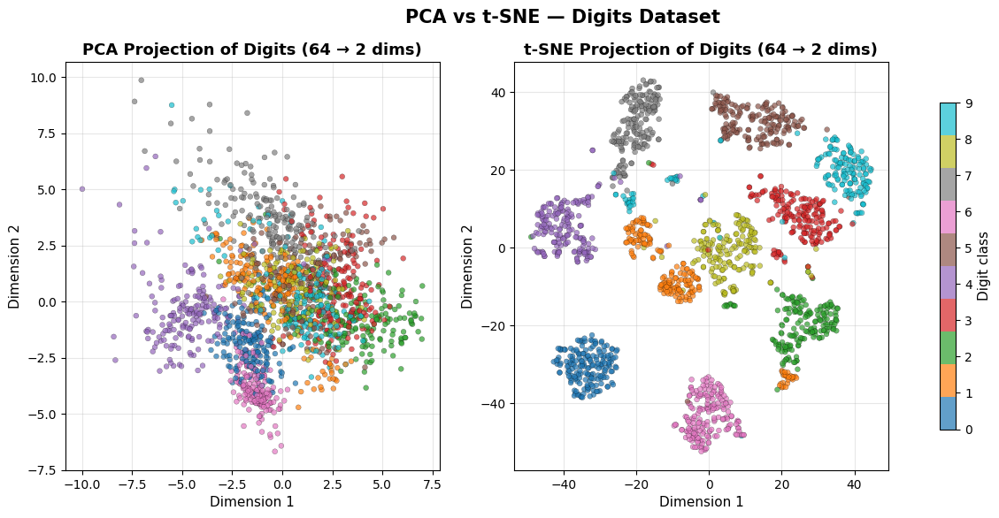
PCA shows a rough separation of digit classes but with significant overlap in the centre. t-SNE resolves all ten digit classes into cleanly separated islands, revealing a level of structure that the linear projection entirely misses.

Effect of Perplexity

perplexities = [5, 30, 50]
fig, axes    = plt.subplots(1, 3, figsize=(18, 5))

for ax, perp in zip(axes, perplexities):
    emb = TSNE(n_components=2, perplexity=perp, max_iter=1000,
               random_state=42).fit_transform(X_sc)
    ax.scatter(emb[:, 0], emb[:, 1], c=y, cmap='tab10',
               alpha=0.65, edgecolors='k', linewidths=0.15, s=16)
    ax.set_title(f'Perplexity = {perp}', fontsize=12, fontweight='bold')
    ax.set_xticks([]); ax.set_yticks([])
    ax.grid(True, alpha=0.2)

plt.suptitle('t-SNE Perplexity Sensitivity — Digits Dataset', fontsize=14, fontweight='bold')
plt.tight_layout()
plt.show()

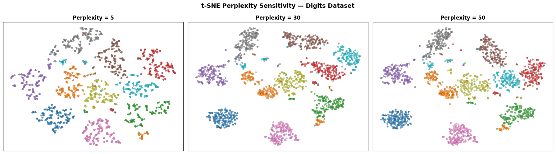
Low perplexity (5) focuses on very local structure and can fragment true clusters. High perplexity (50) brings in more global context. A value of 30 is a good starting point for most datasets.

---

Strengths and Weaknesses

Strengths	Separates clusters with remarkable clarity; handles non-linear manifolds; no assumptions about cluster shape
Weaknesses	Slow — \(O(n^2)\) in the basic algorithm (Barnes-Hut approximation helps); non-deterministic; distances between clusters are not interpretable; cannot be applied to new data without re-running from scratch