4.2.4. Feature Selection

Feature selection is a crucial step in data wrangling. The goal is to retain only those features (inputs) that actually provide meaningful information for modeling or analysis. Removing irrelevant, redundant, or unethical features can improve model performance, reduce computational cost, and prevent biases.

For example, including a feature like religion in a salary prediction model would be both unethical and irrelevant, so it should be excluded.

4.2.4.1. Domain Knowledge

Domain expertise helps identify features that are unlikely to contribute meaningfully to the task. Using prior knowledge allows us to drop irrelevant or sensitive features.

Example: Suppose we are building a model to predict student test scores.

import pandas as pd

df_students = pd.DataFrame({
    "StudentID": [1,2,3,4],
    "Name": ["Alice", "Bob", "Charlie", "Diana"],
    "Age": [16, 17, 16, 18],
    "Gender": ["F", "M", "M", "F"],
    "FavoriteColor": ["Blue", "Green", "Red", "Yellow"],
    "StudyHours": [5, 6, 4, 7],
    "TestScore": [80, 85, 75, 90]
})

# Drop irrelevant or sensitive features
df_students_clean = df_students.drop(columns=["StudentID", "Name", "FavoriteColor", "Gender"])
display(df_students_clean)

	Age	StudyHours	TestScore
0	16	5	80
1	17	6	85
2	16	4	75
3	18	7	90

Here, StudentID, Name, FavoriteColor, and Gender are unlikely to help predict TestScore, so they are removed.

Tip

Domain knowledge is critical for ethical modeling and reducing noise. Always consider the problem context before blindly including features.

4.2.4.2. Statistical Approach

We can also use statistical metrics to select features, based on correlations and redundancy. In section Correlation Heatmaps, we saw how we can plot Correlation Heatmaps to understand our data.

Now we can use them to make decisions.

Among Features

Highly correlated features often carry redundant information. Keeping both may increase model complexity without adding value.

Example: Age vs YearOfBirth

import numpy as np

df = pd.DataFrame({
    "Age": [20, 25, 30, 35, 40],
    "YearOfBirth": [2005, 2000, 1995, 1990, 1985],
    "StudyHours": [20, 21, 30, 28, 15],
    "Score": [80, 85, 90, 95, 82]
})

# Compute correlation
corr_matrix = df.corr()
display(corr_matrix)

	Age	YearOfBirth	StudyHours	Score
Age	1.000000	-1.000000	-0.077254	0.362446
YearOfBirth	-1.000000	1.000000	0.077254	-0.362446
StudyHours	-0.077254	0.077254	1.000000	0.836012
Score	0.362446	-0.362446	0.836012	1.000000

Here, Age and YearOfBirth are perfectly negatively correlated. Keeping both is unnecessary; we can drop one.

With Target

We can calculate feature-target correlation to see how much a feature affects the target. Features with very low correlation can be dropped.

# Correlation with target
feature_target_corr = df.corr()["Score"].sort_values(ascending=False)
display(feature_target_corr)

Score          1.000000
StudyHours     0.836012
Age            0.362446
YearOfBirth   -0.362446
Name: Score, dtype: float64

Features with near-zero correlation are unlikely to improve model performance and can be removed.

Note

Correlation alone is not sufficient. Some features may have non-linear relationships with the target. Consider other metrics or modeling techniques if needed.

4.2.4.3. Dimensionality Reduction

Sometimes datasets contain a large number of features, which can be computationally expensive or non-intuitive. Dimensionality reduction techniques help summarize high-dimensional data into fewer dimensions while preserving meaningful information.

We can apply concepts from Visualizing High-Dimensional Data and identify the features of interest and patterns present in our data.

PCA (Principal Component Analysis)

PCA transforms features into new orthogonal components that explain the maximum variance in the data. It is widely used for both visualization and preprocessing.

import numpy as np
import matplotlib.pyplot as plt
from sklearn.datasets import make_blobs

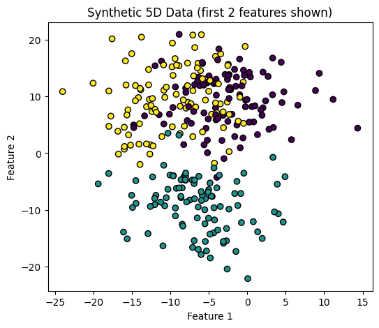
# Generate synthetic dataset with 3 clusters in 5D
X, y = make_blobs(n_samples=300, centers=3, n_features=5, cluster_std=5, random_state=42)

print("Shape of X:", X.shape)   # 300 samples, 5 features
print("Unique clusters in y:", np.unique(y))

# Quick check in 2D (using just first 2 features)
plt.figure(figsize=(6,5))
plt.scatter(X[:,0], X[:,1], c=y, cmap="viridis", edgecolor="k")
plt.xlabel("Feature 1")
plt.ylabel("Feature 2")
plt.title("Synthetic 5D Data (first 2 features shown)")
plt.show()

Shape of X: (300, 5)
Unique clusters in y: [0 1 2]

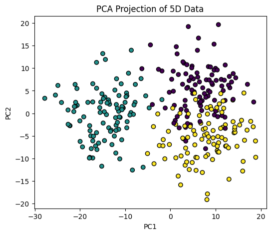
Now we apply PCA to all features.

from sklearn.decomposition import PCA

pca = PCA(n_components=2)
X_pca = pca.fit_transform(X)

plt.figure(figsize=(6,5))
plt.scatter(X_pca[:,0], X_pca[:,1], c=y, cmap="viridis", edgecolor="k")
plt.xlabel("PC1")
plt.ylabel("PC2")
plt.title("PCA Projection of 5D Data")
plt.show()

t-SNE (t-distributed Stochastic Neighbor Embedding)

t-SNE is particularly effective for visualizing high-dimensional data in 2D or 3D while preserving local structure.

# Apply t-SNE
from sklearn.manifold import TSNE

tsne = TSNE(n_components=2, random_state=42, perplexity=30)
X_tsne = tsne.fit_transform(X)

plt.figure(figsize=(6,5))
plt.scatter(X_tsne[:,0], X_tsne[:,1], c=y, cmap="viridis", edgecolor="k")
plt.xlabel("t-SNE 1")
plt.ylabel("t-SNE 2")
plt.title("t-SNE Projection of 5D Data")
plt.show()

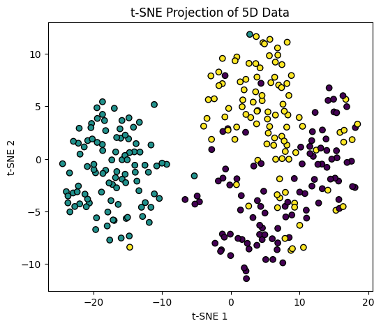
Tip

PCA is faster and preserves global structure, while t-SNE is better at capturing local clusters and patterns. Use them for feature analysis, visualization, or as a preprocessing step before clustering.