6.2.1.2. Linear Regression#
Linear regression is the simplest regression model and the natural starting point for any prediction task. The core idea is elegant: model the target as a weighted sum of the input features.
Imagine you want to predict a house price. You might reason that price goes up by a fixed amount per extra square metre, by another fixed amount per extra bedroom, and by some base amount regardless of other factors. That is linear regression - a straight-line (or hyperplane) relationship between inputs and output.
Because the model is a straight line, it is:
Interpretable - each coefficient directly tells you the marginal effect of a one-unit change in a feature.
Fast - training has a closed-form solution, no iteration needed.
A baseline - always train linear regression first; if it performs well, there is no need for a more complex model.
The Math#
Given \(n\) samples with \(p\) features, the prediction is:
Training minimises the Mean Squared Error over the training set. This has the famous Ordinary Least Squares (OLS) closed-form solution:
The residuals \(e_i = y_i - \hat{y}_i\) should be:
Centred around zero (no systematic bias)
Homoscedastic - constant spread across the range of predictions
Approximately normally distributed
Violations of these assumptions indicate the linear model is mis-specified for the data.
Using Scikit-Learn#
LinearRegression fits OLS with no hyperparameters to tune. After fitting, the learned weights are exposed as .coef_ and .intercept_.
from sklearn.linear_model import LinearRegression

model = LinearRegression()
model.fit(X_train, y_train)
y_pred = model.predict(X_test)
Key attributes:
model.coef_- one weight per featuremodel.intercept_- the bias term \(\beta_0\)
Example#
from sklearn.linear_model import LinearRegression

lr = LinearRegression()
lr.fit(X_train, y_train)

train_r2  = r2_score(y_train, lr.predict(X_train))
test_r2   = r2_score(y_test,  lr.predict(X_test))
test_rmse = np.sqrt(mean_squared_error(y_test, lr.predict(X_test)))

print(f"Train R²  : {train_r2:.3f}")
print(f"Test  R²  : {test_r2:.3f}")
print(f"Test  RMSE: {test_rmse:.1f}")
Train R²  : 0.977
Test  R²  : 0.978
Test  RMSE: 26.2
Linear regression achieves a train \(R^2\) of 0.977 and a test \(R^2\) of 0.978, with an RMSE of 26.2. Because the dataset was generated with a (partially) linear relationship, this is a strong baseline result.
Inspecting the Coefficients#
coef_df = pd.DataFrame({
    "Feature":     [f"Feature {i}" for i in range(X.shape[1])],
    "Coefficient": lr.coef_,
}).sort_values("Coefficient", ascending=False)

fig, ax = plt.subplots(figsize=(9, 4))
colors = ["steelblue" if c > 0 else "tomato" for c in coef_df["Coefficient"]]
ax.barh(coef_df["Feature"], coef_df["Coefficient"], color=colors, edgecolor="black", linewidth=0.6)
ax.axvline(0, color="black", linewidth=0.8)
ax.set_xlabel("Coefficient value", fontsize=12)
ax.set_title("Linear Regression - Learned Coefficients", fontsize=13, fontweight="bold")
ax.grid(True, alpha=0.3, axis="x")
plt.tight_layout()
plt.show()
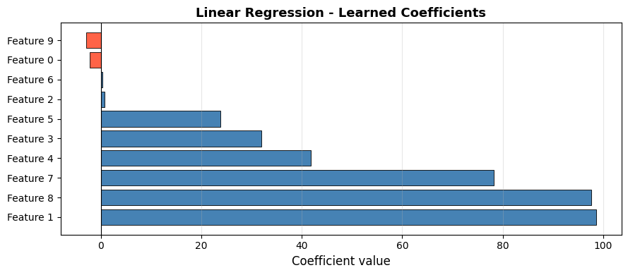
Features with large positive or negative coefficients are the strongest predictors; near-zero coefficients contribute little. Note that 4 of the 10 features are non-informative (by construction), and their coefficients are correspondingly small.
Residual Analysis#
residuals = y_test - lr.predict(X_test)

fig, axes = plt.subplots(1, 2, figsize=(13, 4))

# Residual vs predicted
axes[0].scatter(lr.predict(X_test), residuals, alpha=0.6, edgecolors="k", linewidths=0.4)
axes[0].axhline(0, color="red", linestyle="--", linewidth=1.5)
axes[0].set_xlabel("Predicted value", fontsize=11)
axes[0].set_ylabel("Residual", fontsize=11)
axes[0].set_title("Residual Plot", fontsize=12, fontweight="bold")
axes[0].grid(True, alpha=0.3)

# Distribution of residuals
axes[1].hist(residuals, bins=25, edgecolor="black", alpha=0.8, color="steelblue")
axes[1].set_xlabel("Residual", fontsize=11)
axes[1].set_title("Residual Distribution", fontsize=12, fontweight="bold")
axes[1].grid(True, alpha=0.3)

plt.tight_layout()
plt.show()
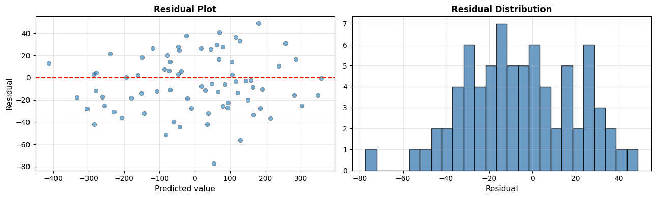
The residuals scatter randomly around zero with no obvious fan-shape, confirming the linear assumption is reasonable for this dataset. The distribution is approximately bell-shaped - another positive sign.
The residual standard deviation is 25.6, which matches the RMSE from above - as expected when residuals are centred at zero.
Strengths and Weaknesses#
Strengths |
Interpretable coefficients; closed-form solution (fast); no hyperparameters; strong baseline |
Weaknesses |
Assumes linearity; sensitive to outliers; degrades with correlated or irrelevant features |
Tip
Always start with Linear Regression. A high \(R^2\) here means the relationship is largely linear and a complex model is unlikely to add much value. A low \(R^2\) motivates exploring non-linear methods.