6.2.3.1. The Perceptron

The perceptron is the atomic building block of every neural network. Before anything else - before layers, before backpropagation, before deep learning - there is one neuron taking inputs, computing a weighted sum, and producing an output.

If you understand the perceptron, you already understand the computation at the heart of every modern neural network.

---

The Core Idea

The perceptron is a direct extension of the models you have already encountered:

Model	Computation	Output
Linear Regression	\(\hat{y} = \mathbf{w}^\top\mathbf{x} + b\)	any real number
Logistic Regression	\(\hat{p} = \sigma(\mathbf{w}^\top\mathbf{x} + b)\)	probability in \((0,1)\)
Perceptron	\(\hat{y} = f(\mathbf{w}^\top\mathbf{x} + b)\)	depends on \(f\)

The only difference is the choice of activation function \(f\). By swapping \(f\) we change what the neuron can output - and this generalisation is exactly what makes neural networks so flexible.

---

The Math

A single perceptron computes two steps:

Step 1 - Pre-activation (linear sum):

\[z = w_1 x_1 + w_2 x_2 + \cdots + w_p x_p + b = \mathbf{w}^\top \mathbf{x} + b\]

This is identical to linear regression: a weighted sum of all input features plus a bias term \(b\).

Step 2 - Activation:

\[\hat{y} = f(z)\]

The activation function \(f\) introduces non-linearity. Common choices:

Activation	Formula	Range	Typical use
Step (original)	\(\mathbf{1}[z \geq 0]\)	\(\{0, 1\}\)	Classic perceptron
Sigmoid	\(\frac{1}{1+e^{-z}}\)	\((0, 1)\)	Output layer, binary
Tanh	\(\frac{e^z - e^{-z}}{e^z + e^{-z}}\)	\((-1, 1)\)	Hidden layers
ReLU	\(\max(0, z)\)	\([0, \infty)\)	Hidden layers (default)

ReLU (Rectified Linear Unit) is the dominant choice for hidden layers today - it is simple, fast, and avoids the vanishing gradient problem that plagues sigmoid and tanh in deep networks (more on this in Deep Learning and Practical Tips).

Learning rule: The perceptron updates its weights after each misclassified training example:

\[\mathbf{w} \leftarrow \mathbf{w} + \eta\,(y_i - \hat{y}_i)\,\mathbf{x}_i\]

where \(\eta\) is the learning rate. This rule converges (for the step activation) if the data are linearly separable - the Perceptron Convergence Theorem. For non-linearly-separable data it will not converge; that is why we need gradient descent and multi-layer networks.

---

In scikit-learn

sklearn.linear_model.Perceptron implements the classic linear perceptron with a step activation. It is equivalent to a linear SVM trained using the perceptron update rule.

from sklearn.linear_model import Perceptron

p = Perceptron(max_iter=1000, eta0=0.1, random_state=42)
p.fit(X_train, y_train)
y_pred = p.predict(X_test)

Key attributes after fitting:

• p.coef_ - weight vector \(\mathbf{w}\) (one row per class in multi-class OvR)

• p.intercept_ - bias terms \(b\)

• p.n_iter_ - number of passes over the data until convergence

Note: The sklearn Perceptron uses the hard step decision; it does not output probabilities. For probability estimates, use LogisticRegression or MLPClassifier.

---

Example

Show code cell source

Hide code cell source

import numpy as np
import pandas as pd
import matplotlib.pyplot as plt
from myst_nb import glue
from sklearn.linear_model import Perceptron
from sklearn.datasets import load_digits
from sklearn.model_selection import train_test_split
from sklearn.preprocessing import StandardScaler
from sklearn.metrics import accuracy_score

np.random.seed(42)

# Shared dataset used throughout all Neural Network pages
data = load_digits()
X, y = data.data, data.target           # 1797 × 64, labels 0–9
X_train, X_test, y_train, y_test = train_test_split(
    X, y, test_size=0.25, random_state=42, stratify=y)

scaler = StandardScaler()
X_train_sc = scaler.fit_transform(X_train)
X_test_sc  = scaler.transform(X_test)

from sklearn.linear_model import Perceptron

p = Perceptron(max_iter=10000, random_state=42)
p.fit(X_train_sc, y_train)

train_acc = accuracy_score(y_train, p.predict(X_train_sc))
test_acc  = accuracy_score(y_test,  p.predict(X_test_sc))

The perceptron achieves a test accuracy of 0.929 - strong for such a simple model, because the digit classes are well-separated in the scaled 64-dimensional pixel space. Train accuracy of 0.966 is close, showing no memorisation.

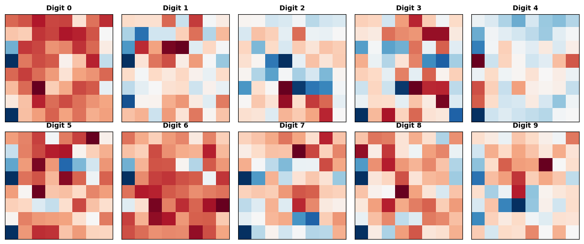
Visualising What the Perceptron Learns

Each of the 10 classes learns its own weight vector — a 64-dimensional template reshaped into an 8×8 image. Pixels with large positive weights push the prediction toward that class; pixels with large negative weights push against it.

Note

This visualisation is a rough sketch — the weight templates from a linear perceptron are noisy and hard to interpret. A deeper network trained with backpropagation would produce much cleaner, more structured weight patterns.

fig, axes = plt.subplots(2, 5, figsize=(12, 5))

for digit, ax in enumerate(axes.ravel()):
    weights = p.coef_[digit].reshape(8, 8)
    ax.imshow(weights, cmap='RdBu_r', interpolation='nearest')
    ax.set_title(f"Digit {digit}", fontsize=10, fontweight='bold')
    ax.set_xticks([])
    ax.set_yticks([])

plt.tight_layout()
plt.show()

The Activation Functions Side by Side

z = np.linspace(-4, 4, 300)

activations = {
    "Step": (z >= 0).astype(float),
    "Sigmoid": 1 / (1 + np.exp(-z)),
    "Tanh": np.tanh(z),
    "ReLU": np.maximum(0, z),
}

fig, axes = plt.subplots(1, 4, figsize=(14, 3.5), sharey=False)

for ax, (name, values) in zip(axes, activations.items()):
    ax.plot(z, values, lw=2.5, color='steelblue')
    ax.axhline(0, color='black', lw=0.7, ls='--')
    ax.axvline(0, color='black', lw=0.7, ls='--')
    ax.set_title(name, fontweight='bold')
    ax.set_xlabel("z")
    ax.grid(True, alpha=0.3)

plt.tight_layout()
plt.show()

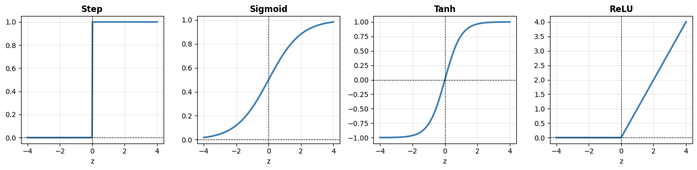
ReLU has zero gradient for \(z < 0\) (the “dead neuron” problem for some neurons) but near-linear gradient for \(z > 0\), making it much easier to train deep networks than sigmoid or tanh, which saturate and kill gradients at both extremes.