6.2.2.2. Logistic Regression#
Logistic Regression is the simplest and most interpretable classification model, and the natural first thing to try on any classification problem. The core idea is to extend the linear prediction from Linear Regression by squashing the output into a probability using the sigmoid function.
Despite its name, this is a classification algorithm. The model learns a linear decision boundary in feature space, making it:
Interpretable - each coefficient is the log-odds change per unit increase in a feature.
Probabilistic - outputs calibrated probability estimates, not just hard class labels.
A strong baseline - always train logistic regression first and beat it before turning to more complex models.
The Math#
The model computes a linear score then passes it through the sigmoid function \(\sigma\):
This maps the unbounded linear output to a probability in \((0, 1)\). The predicted class is:
Training minimises the binary cross-entropy loss:
There is no closed-form solution, so gradient-based optimisation (e.g. L-BFGS) is used. Regularisation (the C hyperparameter) is applied by default: \(C = 1/\lambda\) where \(\lambda\) controls the strength of the \(\ell_2\) penalty.
Key hyperparameters:
Hyperparameter |
Role |
|---|---|
|
Inverse regularisation strength - smaller C → stronger regularisation |
|
|
|
Optimisation algorithm ( |
|
|
In scikit-learn#
from sklearn.linear_model import LogisticRegression
from sklearn.preprocessing import StandardScaler
from sklearn.pipeline import Pipeline

model = Pipeline([
    ('scaler', StandardScaler()),
    ('clf',    LogisticRegression(C=1.0, max_iter=1000, random_state=42))
])
model.fit(X_train, y_train)
y_pred = model.predict(X_test)
y_prob = model.predict_proba(X_test)[:, 1]
Feature scaling is important: gradient descent converges faster when features are on a similar scale.
Example#
from sklearn.linear_model import LogisticRegression
from sklearn.metrics import accuracy_score, roc_auc_score

lr = LogisticRegression(C=1.0, max_iter=1000, random_state=42)
lr.fit(X_train_sc, y_train)

train_acc = accuracy_score(y_train, lr.predict(X_train_sc))
test_acc  = accuracy_score(y_test,  lr.predict(X_test_sc))
test_auc  = roc_auc_score(y_test,   lr.predict_proba(X_test_sc)[:, 1])
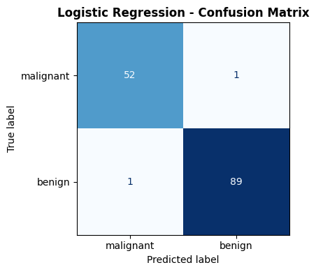
Logistic regression achieves a test accuracy of 0.986 and an AUC-ROC of 0.998. The train accuracy of 0.988 is very close, indicating the model generalises well without overfitting.
Confusion Matrix#
from sklearn.metrics import ConfusionMatrixDisplay, confusion_matrix

cm  = confusion_matrix(y_test, lr.predict(X_test_sc))
fig, ax = plt.subplots(figsize=(5, 4))
ConfusionMatrixDisplay(cm, display_labels=data.target_names).plot(
    ax=ax, colorbar=False, cmap='Blues')
ax.set_title("Logistic Regression - Confusion Matrix", fontweight='bold')
plt.tight_layout()
plt.show()
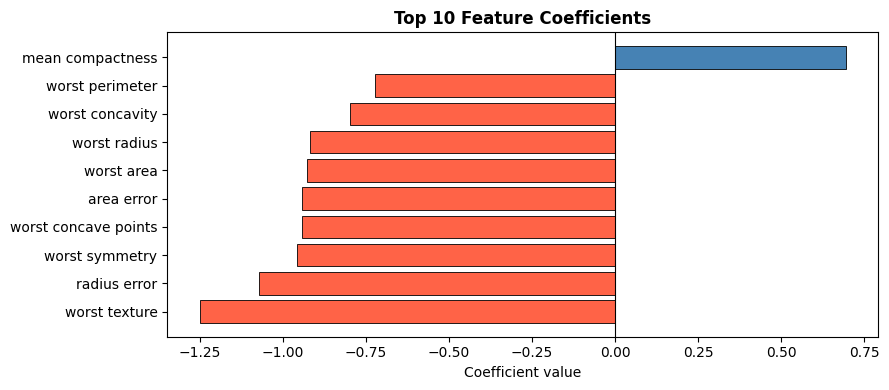
Inspecting Feature Coefficients#
The magnitude of each coefficient reflects its importance to the decision boundary; the sign indicates direction (positive → more likely benign).
coef_df = pd.DataFrame({
    "Feature":    data.feature_names,
    "Coefficient": lr.coef_[0],
}).reindex(pd.Series(lr.coef_[0]).abs().sort_values(ascending=False).index)

top10 = coef_df.head(10)

fig, ax = plt.subplots(figsize=(9, 4))
colors = ["steelblue" if c > 0 else "tomato" for c in top10["Coefficient"]]
ax.barh(top10["Feature"], top10["Coefficient"],
        color=colors, edgecolor="black", linewidth=0.6)
ax.axvline(0, color="black", linewidth=0.8)
ax.set_xlabel("Coefficient value")
ax.set_title("Top 10 Feature Coefficients", fontweight="bold")
plt.tight_layout()
plt.show()