6.1.6. The Bias-Variance Tradeoff#

In the previous section, we explored underfitting and overfitting at a practical level. Now we’ll dig deeper into why this tradeoff exists. The answer lies in one of the most elegant concepts in machine learning: the bias-variance tradeoff.

Understanding this concept will transform you from someone who can train models to someone who truly understands what’s happening under the hood. This is where intuition meets theory!

6.1.6.1. The Fundamental Question#

When your model makes a prediction error, where does that error come from? Is it because:

  • Your model is too simple? (bias)

  • Your model is too sensitive to training data? (variance)

  • The data itself is noisy? (irreducible error)

It turns out all three contribute to your total error, and there’s a beautiful mathematical relationship between them.

import numpy as np
import matplotlib.pyplot as plt
from sklearn.model_selection import train_test_split
from sklearn.preprocessing import PolynomialFeatures
from sklearn.linear_model import LinearRegression
from sklearn.pipeline import make_pipeline
from myst_nb import glue

# Set random seed for reproducibility
np.random.seed(42)

Total Error = Bias² + Variance + Irreducible Error

Think of it as:

  • Bias: How far off is your model on average?

  • Variance: How much does your model jump around?

  • Irreducible: Noise we can’t eliminate

6.1.6.2. Bias: Error from Wrong Assumptions#

Bias is the error introduced by approximating a complex real-world problem with a simplified model.

Think of it this way:

  • You’re trying to catch a baseball

  • But you assume it travels in a straight line (ignoring gravity)

  • Bias = How far off you are on average due to this wrong assumption

In machine learning:

  • High bias = model is too simple = underfitting

  • The model makes systematic errors because it can’t capture the true pattern

def true_function(x):
    """The true underlying pattern (unknown in real problems!)"""
    return 5 + 2*x - 0.3*x**2

# Generate data
X = np.linspace(0, 10, 100).reshape(-1, 1)
y_true = true_function(X.ravel())
y_noisy = y_true + np.random.normal(0, 2, 100)

# Train high-bias model
model_high_bias = LinearRegression()
model_high_bias.fit(X, y_noisy)
y_pred_bias = model_high_bias.predict(X)

Hide code cell source

# Calculate bias visually
plt.figure(figsize=(12, 5))
plt.scatter(X, y_noisy, alpha=0.3, label='Noisy data', s=30)
plt.plot(X, y_true, 'k--', linewidth=3, label='True function', alpha=0.7)
plt.plot(X, y_pred_bias, 'r-', linewidth=2, label='Linear model (high bias)')

sample_points = [20, 50, 80]
for i in sample_points:
    plt.plot([X[i], X[i]], [y_true[i], y_pred_bias[i]],
            'b-', linewidth=2, alpha=0.5)

plt.xlabel('X', fontsize=12)
plt.ylabel('y', fontsize=12)
plt.title('HIGH BIAS: Model Systematically Misses the Pattern', fontsize=14, fontweight='bold')
plt.legend(fontsize=11)
plt.grid(True, alpha=0.3)
plt.tight_layout()
plt.show()
../../../_images/2bffb56feead6071492ad7d1a2d1c3edc295c3b892b31406366624764ec20e1a.png

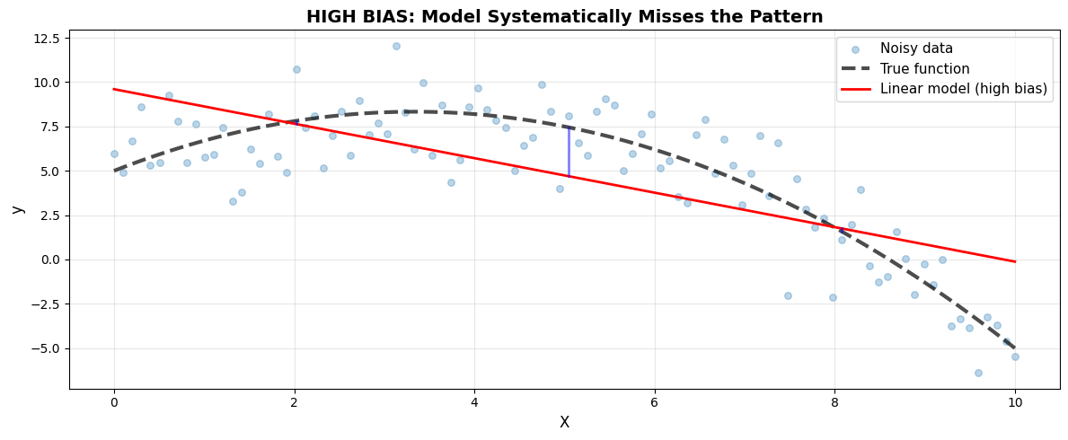
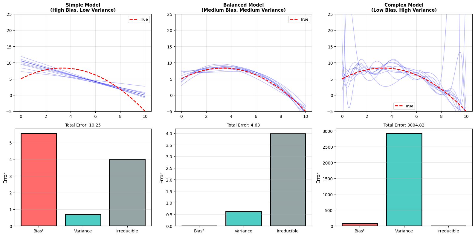
Bias² (squared average error): 5.25

Notice: Linear model ALWAYS underestimates at the edges. This systematic error is BIAS.

Characteristics of High Bias#

High Bias Symptoms:

  • Model too simple for the problem

  • Underfits both training and test data

  • High training error

  • High test error

  • Model makes systematic, predictable errors

  • Adding more data doesn’t help much

Examples:

  • Linear regression on non-linear data

  • Shallow decision tree on complex data

  • Simple rule-based system for complex task

6.1.6.3. Variance: Error from Sensitivity to Training Data#

Variance is the error from the model being too sensitive to small fluctuations in the training data.

Think of it this way:

  • You’re trying to draw the “average” face

  • But you only saw 3 people, and one had a huge nose

  • Now your “average” face has a huge nose!

  • Variance = How much your answer changes based on which examples you saw

In machine learning:

  • High variance = model is too flexible = overfitting

  • The model changes dramatically with different training sets

Hide code cell source

np.random.seed(42)

n_datasets = 10
models = []
predictions = []

fig, axes = plt.subplots(1, 2, figsize=(15, 5))

# Train multiple models on different datasets
for i in range(n_datasets):
    X_sample = np.sort(np.random.uniform(0, 10, 30)).reshape(-1, 1)
    y_sample = true_function(X_sample.ravel()) + np.random.normal(0, 2, 30)

    model_var = make_pipeline(PolynomialFeatures(9), LinearRegression())
    model_var.fit(X_sample, y_sample)

    X_plot = np.linspace(0, 10, 200).reshape(-1, 1)
    y_pred_var = model_var.predict(X_plot)

    predictions.append(y_pred_var)

    axes[0].plot(X_plot, y_pred_var, alpha=0.3, linewidth=1)
    axes[0].scatter(X_sample, y_sample, s=10, alpha=0.3)

axes[0].plot(X_plot, true_function(X_plot.ravel()), 'k--', linewidth=3, label='True function')
axes[0].set_xlabel('X', fontsize=12)
axes[0].set_ylabel('y', fontsize=12)
axes[0].set_title('HIGH VARIANCE: Predictions Jump Around', fontsize=13, fontweight='bold')
axes[0].legend(['True function'] + [f'Model {i+1}' for i in range(3)], fontsize=9)
axes[0].grid(True, alpha=0.3)
axes[0].set_ylim([-10, 30])

predictions = np.array(predictions)
mean_prediction = predictions.mean(axis=0)
variance = predictions.var(axis=0)

# Plot variance
axes[1].plot(X_plot, mean_prediction, 'b-', linewidth=2, label='Average prediction')
axes[1].fill_between(X_plot.ravel(),
                     mean_prediction - np.sqrt(variance),
                     mean_prediction + np.sqrt(variance),
                     alpha=0.3, label='±1 std (variance)')
axes[1].plot(X_plot, true_function(X_plot.ravel()), 'k--', linewidth=2, label='True function')
axes[1].set_xlabel('X', fontsize=12)
axes[1].set_ylabel('y', fontsize=12)
axes[1].set_title('Variance: How Much Predictions Fluctuate', fontsize=13, fontweight='bold')
axes[1].legend(fontsize=10)
axes[1].grid(True, alpha=0.3)
axes[1].set_ylim([-10, 30])

plt.tight_layout()
plt.show()
../../../_images/5e4071be87aede647463dc78637610c4d4bcc480d6226fa5c69f0b1aa6551a1c.png

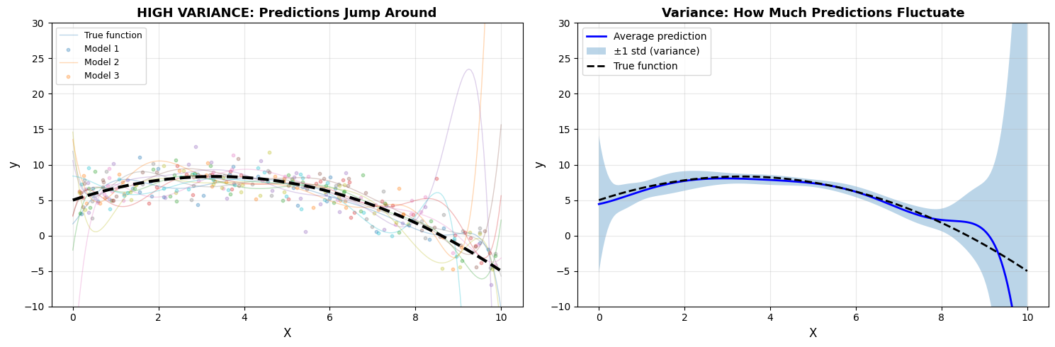
Average variance across predictions: 237.15

Notice: Different training sets → wildly different predictions. This sensitivity is VARIANCE.

Characteristics of High Variance#

High Variance Symptoms:

  • Model too complex/flexible for the data

  • Overfits training data

  • Low training error (fits training data perfectly)

  • High test error (fails on new data)

  • Predictions change drastically with different training sets

  • Large gap between train and test performance

Examples:

  • High-degree polynomial on small dataset

  • Deep decision tree without pruning

  • Neural network with too many parameters

6.1.6.4. The Tradeoff: You Can’t Have Both Low#

Here’s the fundamental insight: You cannot simultaneously minimize both bias and variance.

Why? Because they pull in opposite directions:

  • Reducing bias → Add complexity → Increases variance

  • Reducing variance → Simplify model → Increases bias
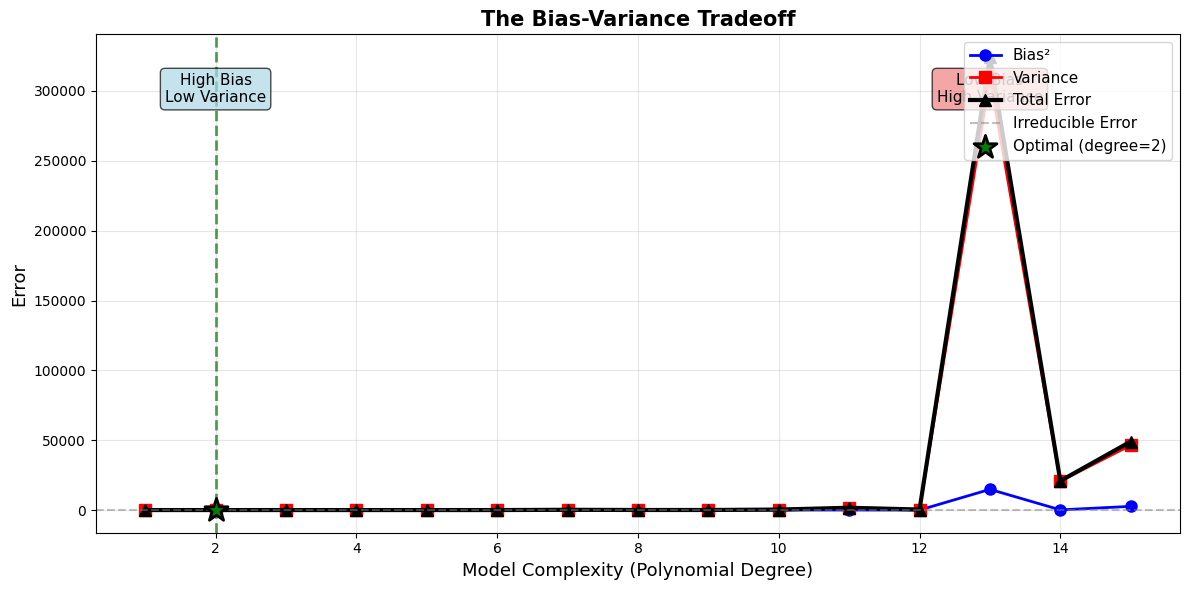
Hide code cell source

degrees = range(1, 16)
n_trials = 20

bias_squared_values = []
variance_values = []
total_error_values = []

# Systematically evaluate bias and variance across complexity levels
for degree in degrees:
    predictions_per_degree = []

    for trial in range(n_trials):
        X_train = np.sort(np.random.uniform(0, 10, 30)).reshape(-1, 1)
        y_train = true_function(X_train.ravel()) + np.random.normal(0, 2, 30)

        model = make_pipeline(PolynomialFeatures(degree), LinearRegression())
        model.fit(X_train, y_train)

        X_test = np.linspace(0, 10, 50).reshape(-1, 1)
        y_pred = model.predict(X_test)
        predictions_per_degree.append(y_pred)

    predictions_per_degree = np.array(predictions_per_degree)

    y_true_test = true_function(X_test.ravel())

    # Calculate bias and variance
    mean_prediction = predictions_per_degree.mean(axis=0)
    bias_squared = np.mean((mean_prediction - y_true_test)**2)
    variance = np.mean(predictions_per_degree.var(axis=0))

    irreducible_error = 4.0

    total_error = bias_squared + variance + irreducible_error

    bias_squared_values.append(bias_squared)
    variance_values.append(variance)
    total_error_values.append(total_error)

plt.figure(figsize=(12, 6))

plt.plot(degrees, bias_squared_values, 'b-o', linewidth=2, markersize=8, label='Bias²')
plt.plot(degrees, variance_values, 'r-s', linewidth=2, markersize=8, label='Variance')
plt.plot(degrees, total_error_values, 'k-^', linewidth=3, markersize=8, label='Total Error')
plt.axhline(y=irreducible_error, color='gray', linestyle='--', alpha=0.5, label='Irreducible Error')

optimal_idx = np.argmin(total_error_values)
optimal_degree = degrees[optimal_idx]
plt.axvline(x=optimal_degree, color='green', linestyle='--', alpha=0.7, linewidth=2)
plt.scatter([optimal_degree], [total_error_values[optimal_idx]],
           s=300, c='green', marker='*', edgecolors='black', linewidths=2,
           label=f'Optimal (degree={optimal_degree})', zorder=5)

plt.text(2, max(total_error_values)*0.9, 'High Bias\nLow Variance',
        fontsize=11, ha='center', bbox=dict(boxstyle='round', facecolor='lightblue', alpha=0.7))
plt.text(13, max(total_error_values)*0.9, 'Low Bias\nHigh Variance',
        fontsize=11, ha='center', bbox=dict(boxstyle='round', facecolor='lightcoral', alpha=0.7))

plt.xlabel('Model Complexity (Polynomial Degree)', fontsize=13)
plt.ylabel('Error', fontsize=13)
plt.title('The Bias-Variance Tradeoff', fontsize=15, fontweight='bold')
plt.legend(fontsize=11, loc='upper right')
plt.grid(True, alpha=0.3)
plt.tight_layout()
plt.show()
../../../_images/75329a8386a81534f54526cf6ebc62818d4df84112f8c67794ad63d6896d624c.png

Key Observations:

  1. As complexity increases, bias² decreases (better fit)

  2. As complexity increases, variance increases (less stable)

  3. Total error = Bias² + Variance + Irreducible

  4. Optimal complexity: 2 (minimizes total error)

  5. Can’t reduce both simultaneously - it’s a TRADEOFF

The Mathematical Decomposition#

Important

Error Decomposition Formula:

For a model’s prediction \(\hat{f}(x)\) compared to true value \(y\):

\[\text{Expected Error} = \text{Bias}^2 + \text{Variance} + \text{Irreducible Error}\]

Where:

  • Bias² = \((E[\hat{f}(x)] - f(x))^2\)

    • How far is the average prediction from the truth?

  • Variance = \(E[(\hat{f}(x) - E[\hat{f}(x)])^2]\)

    • How much do predictions vary across training sets?

  • Irreducible Error = Noise in the data itself (cannot be reduced)
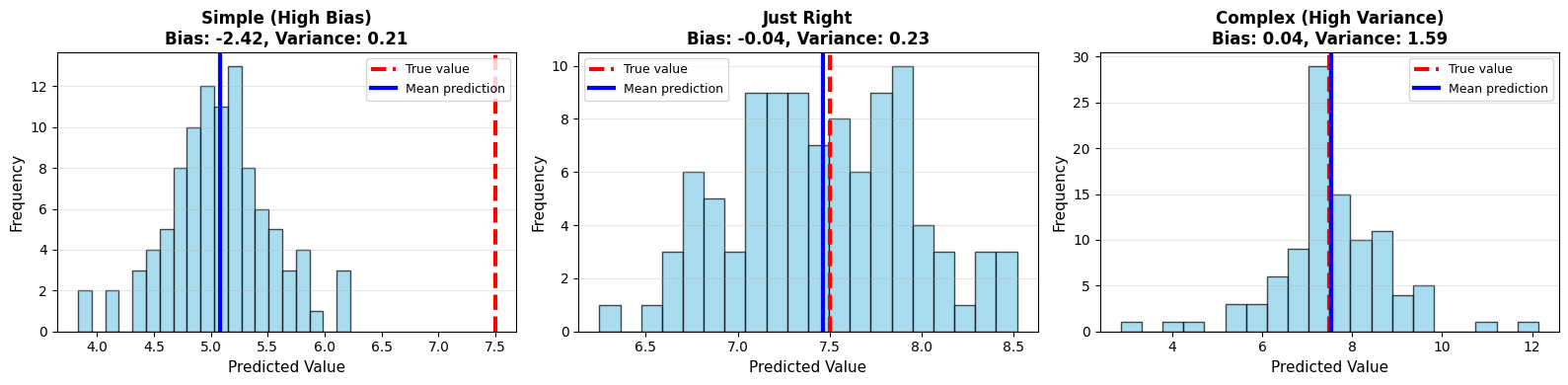
Hide code cell source

np.random.seed(42)
x_point = 5.0
y_true_point = true_function(np.array([x_point]))[0]

simple_predictions = []
optimal_predictions = []
complex_predictions = []

# Evaluate predictions at a single point across multiple training sets
for trial in range(100):
    X_train = np.sort(np.random.uniform(0, 10, 30)).reshape(-1, 1)
    y_train = true_function(X_train.ravel()) + np.random.normal(0, 2, 30)

    for degree, pred_list in [(1, simple_predictions),
                               (2, optimal_predictions),
                               (10, complex_predictions)]:
        model = make_pipeline(PolynomialFeatures(degree), LinearRegression())
        model.fit(X_train, y_train)
        pred = model.predict([[x_point]])[0]
        pred_list.append(pred)

fig, axes = plt.subplots(1, 3, figsize=(16, 4))

for ax, preds, title, degree in zip(axes,
                                     [simple_predictions, optimal_predictions, complex_predictions],
                                     ['Simple (High Bias)', 'Just Right', 'Complex (High Variance)'],
                                     [1, 2, 10]):
    ax.hist(preds, bins=20, alpha=0.7, color='skyblue', edgecolor='black')
    ax.axvline(y_true_point, color='red', linewidth=3, label='True value', linestyle='--')
    ax.axvline(np.mean(preds), color='blue', linewidth=3, label='Mean prediction', linestyle='-')

    bias = np.mean(preds) - y_true_point
    variance = np.var(preds)

    ax.set_xlabel('Predicted Value', fontsize=11)
    ax.set_ylabel('Frequency', fontsize=11)
    ax.set_title(f'{title}\nBias: {bias:.2f}, Variance: {variance:.2f}',
                fontsize=12, fontweight='bold')
    ax.legend(fontsize=9)
    ax.grid(True, alpha=0.3, axis='y')

plt.tight_layout()
plt.show()
../../../_images/90a7a0d3b8656dcc3b6ca56a600dc933b5ea9be10855d35667c163daf0e62bb3.png

At x = 5:

True value: 7.50

Simple model (degree 1):

  • Mean prediction: 5.08

  • Bias: -2.42

  • Variance: 0.21

Optimal model (degree 2):

  • Mean prediction: 7.46

  • Bias: -0.04

  • Variance: 0.23

Complex model (degree 10):

  • Mean prediction: 7.54

  • Bias: 0.04

  • Variance: 1.59

6.1.6.5. Connection to Model Complexity#

The bias-variance tradeoff is intimately connected to model complexity:

Model Type

Complexity

Bias

Variance

Best For

Simple (linear)

Low

High

Low

Simple patterns, small data

Medium (quadratic)

Medium

Medium

Medium

Moderate patterns, medium data

Complex (high-degree)

High

Low

High

Complex patterns, large data

Hide code cell source

# Visualize predictions from multiple models

fig, axes = plt.subplots(2, 3, figsize=(16, 8))

degrees_to_show = [1, 3, 10]
titles = ['Simple Model\n(High Bias, Low Variance)',
         'Balanced Model\n(Medium Bias, Medium Variance)',
         'Complex Model\n(Low Bias, High Variance)']

for col, (degree, title) in enumerate(zip(degrees_to_show, titles)):
    ax_top = axes[0, col]

    # Train multiple models and plot predictions
    for trial in range(10):
        X_sample = np.sort(np.random.uniform(0, 10, 30)).reshape(-1, 1)
        y_sample = true_function(X_sample.ravel()) + np.random.normal(0, 2, 30)

        model = make_pipeline(PolynomialFeatures(degree), LinearRegression())
        model.fit(X_sample, y_sample)

        X_plot = np.linspace(0, 10, 200).reshape(-1, 1)
        y_pred = model.predict(X_plot)

        ax_top.plot(X_plot, y_pred, alpha=0.3, linewidth=1, color='blue')

    ax_top.plot(X_plot, true_function(X_plot.ravel()), 'r--', linewidth=2, label='True')
    ax_top.set_title(title, fontsize=11, fontweight='bold')
    ax_top.set_ylim([-5, 25])
    ax_top.grid(True, alpha=0.3)
    ax_top.legend(fontsize=9)

    ax_bottom = axes[1, col]

    # Calculate bias and variance
    predictions = []
    for trial in range(50):
        X_sample = np.sort(np.random.uniform(0, 10, 30)).reshape(-1, 1)
        y_sample = true_function(X_sample.ravel()) + np.random.normal(0, 2, 30)

        model = make_pipeline(PolynomialFeatures(degree), LinearRegression())
        model.fit(X_sample, y_sample)

        X_test = np.linspace(0, 10, 50).reshape(-1, 1)
        y_pred = model.predict(X_test)
        predictions.append(y_pred)

    predictions = np.array(predictions)
    mean_pred = predictions.mean(axis=0)
    y_true_test = true_function(X_test.ravel())

    bias_sq = np.mean((mean_pred - y_true_test)**2)
    var = np.mean(predictions.var(axis=0))
    irreducible = 4.0
    total = bias_sq + var + irreducible

    components = [bias_sq, var, irreducible]
    labels = ['Bias²', 'Variance', 'Irreducible']
    colors = ['#FF6B6B', '#4ECDC4', '#95A5A6']

    ax_bottom.bar(labels, components, color=colors, edgecolor='black', linewidth=2)
    ax_bottom.set_ylabel('Error', fontsize=11)
    ax_bottom.set_title(f'Total Error: {total:.2f}', fontsize=10)
    ax_bottom.grid(True, alpha=0.3, axis='y')

plt.tight_layout()
plt.show()
../../../_images/ae4d574314d2a7175452ae9de1eab45e19ae61c08cad84c02a142513bf38b661.png

6.1.6.6. The No Free Lunch Theorem#

The bias-variance tradeoff leads to an important realization: There is no universally best model.

The No Free Lunch Theorem states: Averaged over all possible problems, every algorithm performs equally well.

What this means practically:

  • Simple models win on simple problems

  • Complex models win on complex problems

  • You need to match model complexity to problem complexity

  • Always validate on your specific data!

Hide code cell source

from sklearn.tree import DecisionTreeRegressor
from sklearn.ensemble import RandomForestRegressor
from sklearn.svm import SVR

problems = [
    {
        'name': 'Simple Linear',
        'func': lambda x: 2*x + 3,
        'best_model': 'Linear Regression'
    },
    {
        'name': 'Complex Non-Linear',
        'func': lambda x: 10*np.sin(x) + 0.5*x**2,
        'best_model': 'Random Forest'
    }
]

models = {
    'Linear': LinearRegression(),
    'Tree': DecisionTreeRegressor(max_depth=5, random_state=42),
    'Forest': RandomForestRegressor(n_estimators=50, max_depth=10, random_state=42)
}

fig, axes = plt.subplots(2, 2, figsize=(14, 10))

for prob_idx, problem in enumerate(problems):
    # Generate data for each problem
    X = np.sort(np.random.uniform(0, 10, 100)).reshape(-1, 1)
    y = problem['func'](X.ravel()) + np.random.normal(0, 1, 100)

    X_train, X_test = X[:70], X[70:]
    y_train, y_test = y[:70], y[70:]

    # Plot data
    ax_data = axes[prob_idx, 0]
    ax_data.scatter(X_train, y_train, alpha=0.6, s=40, label='Train')
    ax_data.scatter(X_test, y_test, alpha=0.6, s=60, marker='s', label='Test')
    ax_data.plot(X, problem['func'](X.ravel()), 'k--', linewidth=2, label='True')
    ax_data.set_title(f"Problem: {problem['name']}", fontsize=12, fontweight='bold')
    ax_data.legend()
    ax_data.grid(True, alpha=0.3)

    ax_results = axes[prob_idx, 1]
    model_names = []
    test_errors = []

    # Train and evaluate each model
    for name, model in models.items():
        model.fit(X_train, y_train)
        y_pred = model.predict(X_test)
        mse = np.mean((y_test - y_pred)**2)

        model_names.append(name)
        test_errors.append(mse)

    colors = ['green' if name == problem['best_model'].split()[0] else 'gray'
             for name in model_names]

    ax_results.bar(model_names, test_errors, color=colors, edgecolor='black', linewidth=2)
    ax_results.set_ylabel('Test MSE', fontsize=11)
    ax_results.set_title(f'Best: {problem["best_model"]}', fontsize=11, fontweight='bold')
    ax_results.grid(True, alpha=0.3, axis='y')

plt.tight_layout()
plt.show()
../../../_images/4a66a8e89f3c2575685eee0859bb9e1168c4206e21880b14ebba956516022495.png

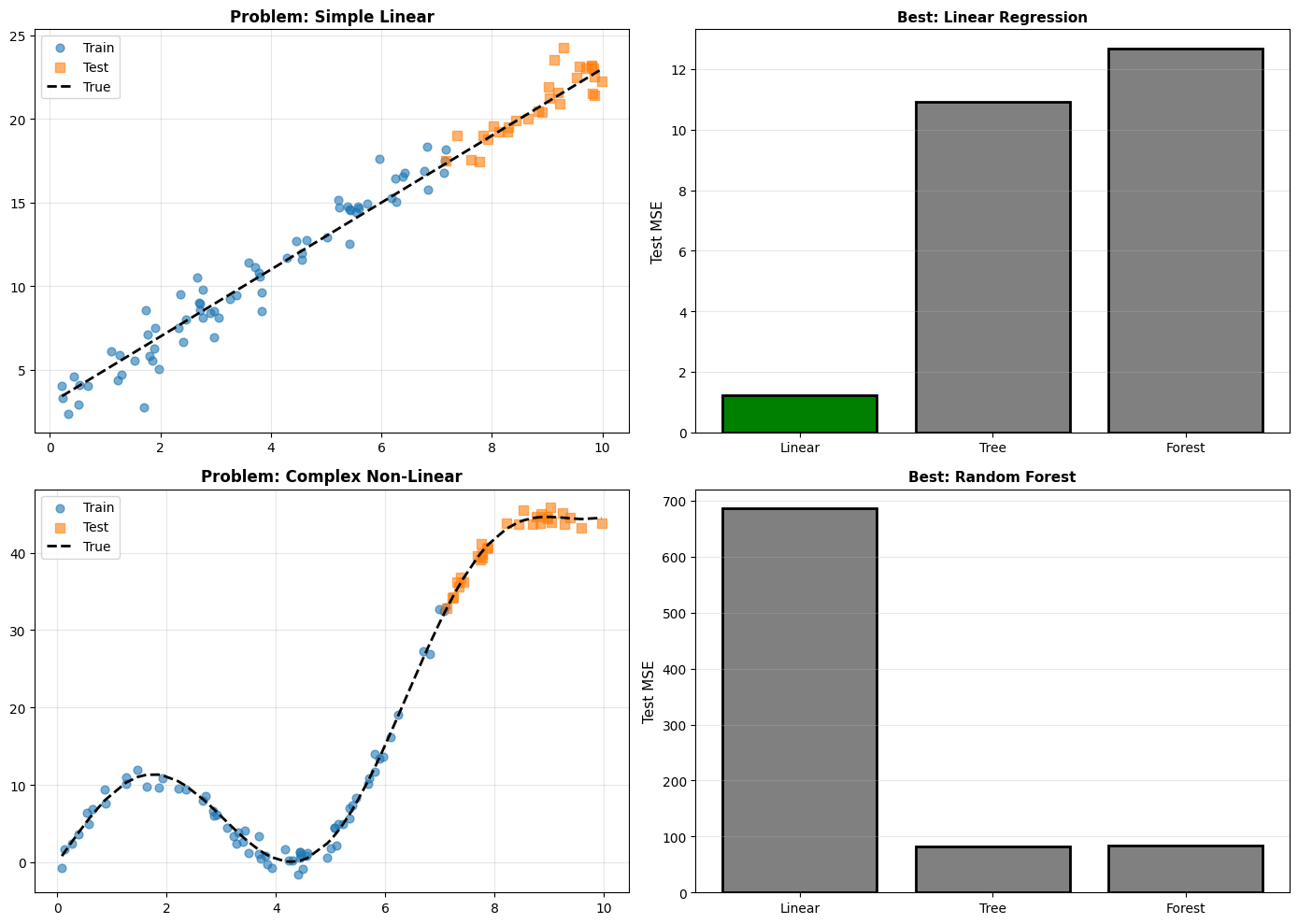
No Free Lunch Theorem in Action:

  • Linear problem → Linear model wins

  • Complex problem → Complex model wins

  • No single ‘best’ model for all problems

  • Must validate on YOUR specific data!

6.1.6.7. Practical Implications#

Tip

How to Navigate the Bias-Variance Tradeoff:

  1. Start simple - Begin with low-complexity models

  2. Monitor both - Track training AND validation error

  3. Increase complexity gradually - Add just enough

  4. Use validation - Catch overfitting early

  5. Regularization helps - Controls variance without sacrificing too much bias

  6. More data helps variance - Large datasets allow complex models

  7. Feature engineering helps bias - Better features reduce need for complexity

Practical Decision Guide:

Situation 1: High training error + High test error

  • High BIAS (underfitting)

  • Solution: Increase model complexity

  • Example: Try polynomial features, deeper tree, more layers

Situation 2: Low training error + High test error

  • High VARIANCE (overfitting)

  • Solution: Reduce complexity OR get more data

  • Example: Add regularization, prune tree, dropout, early stopping

Situation 3: Large gap between training and test

  • High VARIANCE

  • Model is memorizing rather than learning

Situation 4: Both errors decreasing with more data

  • You’re on the right track!

  • More data will help

Situation 5: Both errors plateau despite more data

  • High BIAS

  • Need more model capacity, not more data

Warning

Don’t Oversimplify!

While the bias-variance tradeoff is a powerful mental model, remember:

  • Real models have many sources of error

  • The tradeoff isn’t always perfect (regularization can help both!)

  • Always validate empirically on your data