Embeddings Primer

Supplementary Material for RAG Architecture

CIS 6930 - Data Engineering with LLMs

---

Why Embeddings?

RAG requires converting text to vectors for similarity search.

The problem: Computers work with numbers, not words.

The solution: Map text to dense numerical vectors where:

• Similar meanings → nearby vectors
• Different meanings → distant vectors

This enables semantic search beyond keyword matching.

---

Roadmap: From Words to Embeddings

Era	Method	Key Idea
1990s	One-Hot Encoding	Binary vectors, no semantics
2000s	TF-IDF	Term importance weighting
2013	Word2Vec	Learn from context
2018+	Transformers	Contextual embeddings
Now	Sentence Transformers	Full sentence meaning

---

One-Hot Encoding

Simplest approach: Each word gets a unique binary vector.

Word	Vector
dog	[1, 0, 0, 0, 0, 0, 0]
cat	[0, 1, 0, 0, 0, 0, 0]
person	[0, 0, 1, 0, 0, 0, 0]
holding	[0, 0, 0, 1, 0, 0, 0]

Problems:

• No semantic similarity (dog and cat equally different from “tree”)
• Vectors are huge (vocabulary size)
• Sparse and inefficient

Slide adapted from V. Ordonez

---

Bag-of-Words Representation

Represent documents by word counts:

Document	dog	cat	person	holding	tree
“person holding dog”	1	0	1	1	0
“person holding cat”	0	1	1	1	0

Still no semantics: “dog” and “cat” treated as completely unrelated.

Slide adapted from V. Ordonez

---

The Distributional Hypothesis

“You shall know a word by the company it keeps.” — J.R. Firth, 1957

Key insight: Words that appear in similar contexts have similar meanings.

• “The cat sat on the mat”
• “The dog sat on the mat”

Both “cat” and “dog” appear in the same context → they must be semantically related.

Lenci (2008) - Distributional Semantics

---

Document Frequency: Rare vs Common Terms

Intuition: Rare terms are more informative than common terms.

Term	Appears In	Informativeness
“the”	99% of docs	Very low
“algorithm”	5% of docs	Medium
“arachnocentric”	0.001% of docs	Very high

If a query contains “arachnocentric” and a document contains it, that document is likely relevant.

---

TF-IDF: Term Frequency × Inverse Document Frequency

TF (Term Frequency): How often does the term appear in this document?

\[\text{TF}(t, d) = \frac{\text{count of } t \text{ in } d}{\text{total terms in } d}\]

IDF (Inverse Document Frequency): How rare is this term across all documents?

\[\text{IDF}(t) = \log\left(\frac{N}{\text{df}_t}\right)\]

TF-IDF:

\[\text{TF-IDF}(t, d) = \text{TF}(t, d) \times \text{IDF}(t)\]

---

TF-IDF in Python

from sklearn.feature_extraction.text import TfidfVectorizer

corpus = [
    "The quick brown fox jumps over the lazy dog",
    "The dog barks at the fox",
    "The fox is quick and clever"
]

vectorizer = TfidfVectorizer()
tfidf_matrix = vectorizer.fit_transform(corpus)

# Get feature names (vocabulary)
print(vectorizer.get_feature_names_out())
# ['and', 'at', 'barks', 'brown', 'clever', 'dog', ...]

# Each row is a document vector
print(tfidf_matrix.toarray())

---

Word2Vec: Learning from Context

Key idea: Predict surrounding words from a center word (or vice versa).

Two architectures:

• CBOW: Predict center word from context
• Skip-gram: Predict context from center word

"The cat sat on the floor"

CBOW: [the, sat, on, the] → predict "cat"
Skip-gram: "sat" → predict [the, cat, on, the]

Mikolov et al. (2013) - Word2Vec

---

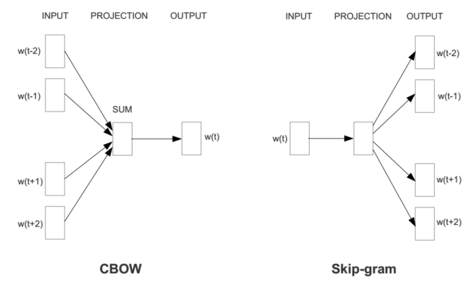
CBOW vs Skip-gram

CBOW (Continuous Bag of Words):

• Input: context words (surrounding words)
• Output: predict the center word
• Faster to train
• Better for frequent words

Skip-gram:

• Input: center word
• Output: predict context words
• Slower but more accurate
• Better for rare words and small datasets

Mikolov et al. (2013) - Word2Vec

---

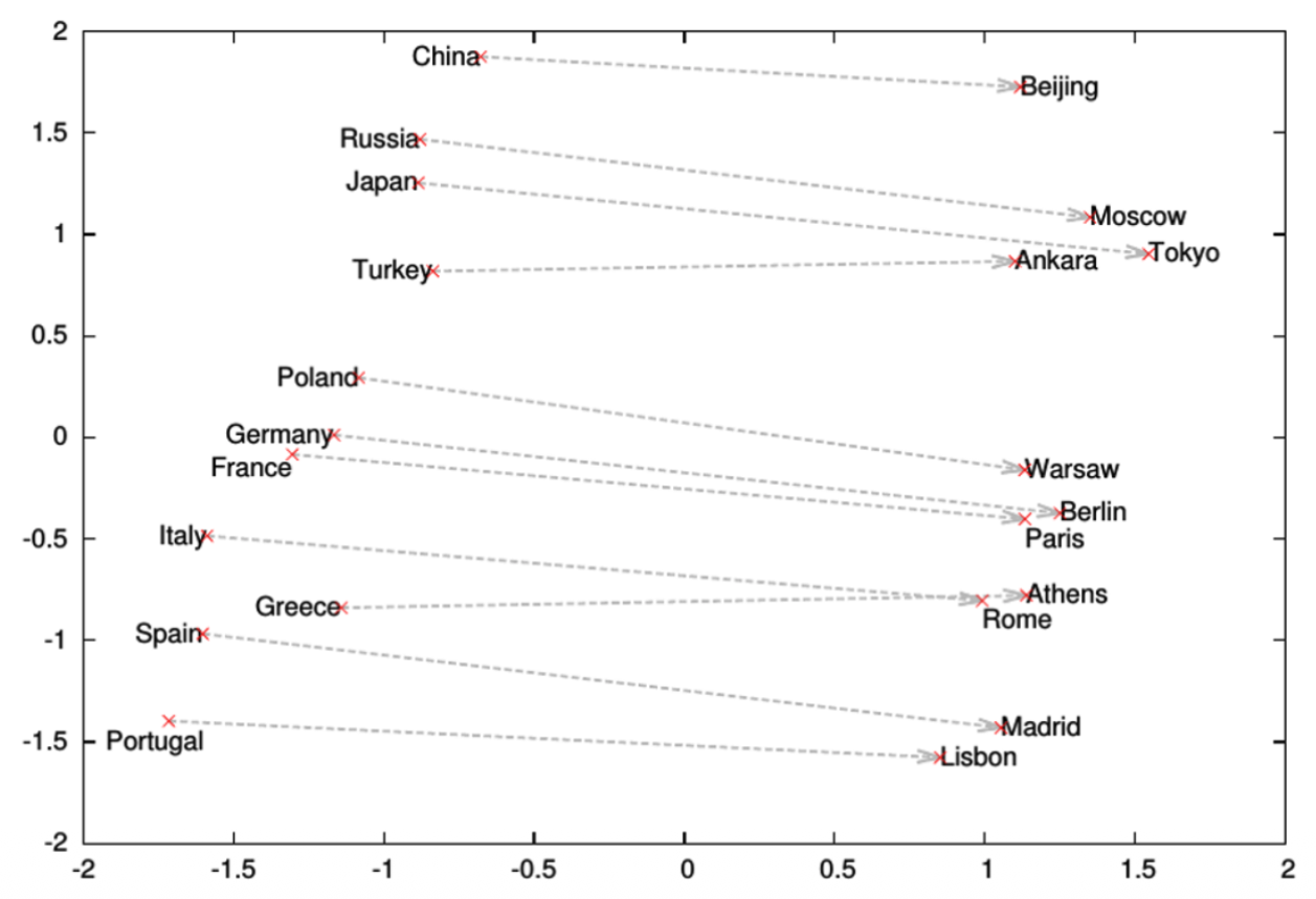
Word2Vec: The Interesting Result

Word vectors capture semantic relationships through arithmetic:

\[\vec{king} - \vec{man} + \vec{woman} \approx \vec{queen}\]

More examples:

• Paris - France + Italy ≈ Rome
• Bigger - Big + Small ≈ Smaller

The learned vectors encode analogical relationships. These relationships are approximate and depend on the training corpus.

Mikolov et al. (2013) - Word2Vec

---

From Words to Sentences

Problem: Word2Vec gives word vectors, but RAG needs document/chunk vectors.

Simple solution: Average the word vectors.

def document_vector(doc, word2vec_model):
    words = doc.split()
    vectors = [word2vec_model[w] for w in words if w in word2vec_model]
    return np.mean(vectors, axis=0)

Better solution: Use models trained for sentence similarity.

---

Sentence Transformers (2019+)

SBERT (Sentence-BERT): Fine-tune BERT for sentence similarity.

from sentence_transformers import SentenceTransformer

model = SentenceTransformer('all-MiniLM-L6-v2')

sentences = [
    "The cat sat on the mat",
    "A feline rested on the rug",
    "The stock market crashed today"
]

embeddings = model.encode(sentences)
# embeddings.shape: (3, 384)

Sentences 1 and 2 will have high cosine similarity; sentence 3 will be distant.

---

Measuring Similarity: Cosine Similarity

Cosine similarity: Measures angle between vectors (ignores magnitude).

\[\cos(\theta) = \frac{\vec{A} \cdot \vec{B}}{||\vec{A}|| \times ||\vec{B}||}\]

from sklearn.metrics.pairwise import cosine_similarity

# Compare two embeddings
similarity = cosine_similarity([emb1], [emb2])[0][0]
# Range: -1 (opposite) to 1 (identical)

For RAG: Higher cosine similarity = more relevant document.

---

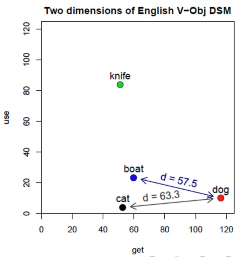
Euclidean Distance

Euclidean Distance:

• Measures straight-line distance
• Affected by vector magnitude

Example: Using dimensions “use” and “get”:

• Distance(boat, dog) = 57.5
• Distance(cat, dog) = 63.3

Boat appears closer to dog than cat does, which is counterintuitive for semantic similarity.

---

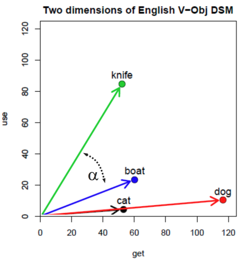
Cosine Similarity

Cosine Similarity:

• Measures angle between vectors
• Ignores magnitude (normalized)

Example: Same words, same dimensions:

• Cat and dog have a small angle between them
• Cosine similarity correctly identifies their semantic relationship

Normalization removes the effect of word frequency, making cat and dog similar regardless of how often they appear.

---

Why Cosine for Text Similarity?

For text similarity: Cosine similarity is preferred because document length shouldn’t affect similarity.

• A short document about “dogs” should match a long document about “dogs”
• Euclidean distance would penalize the length difference
• Cosine similarity focuses on the direction (meaning), not magnitude (length)

Slides from Louis-Philippe Morency

---

Embedding Models for RAG

Model	Dimensions	Speed	Quality
all-MiniLM-L6-v2	384	Fast	Good
all-mpnet-base-v2	768	Medium	Better
text-embedding-3-small (OpenAI)	1536	API	Excellent
text-embedding-3-large (OpenAI)	3072	API	Best

Trade-off: Larger embeddings = better quality but slower search and more storage.

---

Using Embeddings in RAG

from sentence_transformers import SentenceTransformer

model = SentenceTransformer('all-MiniLM-L6-v2')

# 1. Embed your documents (offline)
doc_embeddings = model.encode(documents)

# 2. Embed the query (online)
query_embedding = model.encode(query)

# 3. Find most similar documents
similarities = cosine_similarity([query_embedding], doc_embeddings)[0]
top_k_indices = similarities.argsort()[-k:][::-1]
relevant_docs = [documents[i] for i in top_k_indices]

---

Summary

1. Embeddings convert text to dense vectors
2. TF-IDF weights terms by importance (sparse)
3. Word2Vec learns from context (dense, word-level)
4. Sentence Transformers encode full sentences (dense, sentence-level)
5. Cosine similarity measures semantic relatedness
6. RAG uses embeddings for semantic retrieval

For Assignment 2: You’ll use sentence-transformers to embed chunks and queries.

---

References

• Mikolov et al. (2013) - Word2Vec
• Reimers & Gurevych (2019) - Sentence-BERT
• MTEB Leaderboard - Embedding model benchmarks

Slides adapted from L.P. Morency, V. Hristidis, V. Ordonez</div>